Nomenclaturas de las Unidades Territoriales Estadísticas (NUTS)
Las Nomenclaturas de las Unidades Territoriales Estadísticas (NUTS por sus siglas en Francés) son el conjunto de demarcaciones territoriales de la Unión Europea creada por Eurostat que se utiliza con fines estadísticos y analíticos. Su establecimiento se basa, en principio, en función de las unidades administrativas que operan en cada uno de los Estados miembros. Es decir, las regiones geográficas se basan en las entidades con autoridades administrativas en cada uno de los países que conforman la región Euro. Los niveles NUTS en los que se divide cada uno de dichas unidades administrativas dependen, principalmente, de ciertos límites mínimos y máximos de población.
La actual clasificación NUTS, válida desde 2018, se enumera en 104 regiones en NUTS-1, 281 regiones en NUTS-2 y 1348 regiones en NUTS 3. En España, por ejemplo, el NUTS-1 corresponde a grupos de regiones (17), el NUTS-2 se configura en torno a las Comunidades Autónomas y Ciudades Autónomas (19) y el NUTS-3 se compone de las Provincias, Consejos Insulares y Cabildos (59). Se puede consultar las regiones NUTS de cada país en el siguiente enlace de Eurostat.
A efectos prácticos utilizaremos la función get_eurostat_geospatial() para descargar la información geográfica de Gisco, el organismo responsable de generar y actualizar la información geográfica de la Comisión Europea. El paquete get_eurostat_geospatial() descarga tres tipos de información: sf, spdf y df, como veremos en los siguientes subapartados.
Antes de empezar la exposición cargamos algunos paquetes que utilizaremos a lo largo del post.
library(eurostat)
library(tidyverse)
library(sf)
library(DT)
library(cowplot)
library(RColorBrewer)
Simple feature (sf)
Como se expone aquí, simple feature o simple feature access hace referencia al International Organization for Standarization (ISO 19125) que describe y especifica cómo los objetos en el mundo real pueden ser representados en las computadoras, con especial énfasis a los objetos espaciales geométricos. Por tanto, definen un modelo común de geometrías de dos dimensiones que se utilizan en los sistemas de información geográfica.
Por consiguiente, para realizar mapas base a cada uno de los niveles NUTS podemos obtener en primer lugar el sf con la función get_eurostat_geospatial() y representar el mapa al nivel deseado utilizando los siguientes comandos:
NUTS-0
# NUTS-0
mapdata_0 <- get_eurostat_geospatial(nuts_level = 0)
head(mapdata_0)
## Simple feature collection with 6 features and 7 fields
## geometry type:  MULTIPOLYGON
## dimension:      XY
## bbox:           xmin: 2.54601 ymin: 34.56908 xmax: 34.56859 ymax: 51.50246
## geographic CRS: WGS 84
##   id CNTR_CODE                                                        NUTS_NAME
## 1 BG        BG <U+0411><U+042A><U+041B><U+0413><U+0410><U+0420><U+0418><U+042F>
## 2 CH        CH                                          SCHWEIZ/SUISSE/SVIZZERA
## 3 CY        CY                        <U+039A><U+03A5><U+03A0><U+03A1><U+039F>S
## 4 AL        AL                                                        SHQIPËRIA
## 5 CZ        CZ                                                  CESKÁ REPUBLIKA
## 6 BE        BE                                                 BELGIQUE-BELGIË
##   LEVL_CODE FID NUTS_ID                       geometry geo
## 1         0  BG      BG MULTIPOLYGON (((22.99717 43...  BG
## 2         0  CH      CH MULTIPOLYGON (((8.61383 47....  CH
## 3         0  CY      CY MULTIPOLYGON (((33.75237 34...  CY
## 4         0  AL      AL MULTIPOLYGON (((19.831 42.4...  AL
## 5         0  CZ      CZ MULTIPOLYGON (((14.49122 51...  CZ
## 6         0  BE      BE MULTIPOLYGON (((5.10218 51....  BE

mapdata_0 %>%
  ggplot(., aes()) +
  geom_sf(fill="purple", color="white", size = 0.1) +
  theme_minimal() +
  xlim(c(-30, 44)) +
  ylim(c(35, 75)) +
  ggtitle("NUTS-0")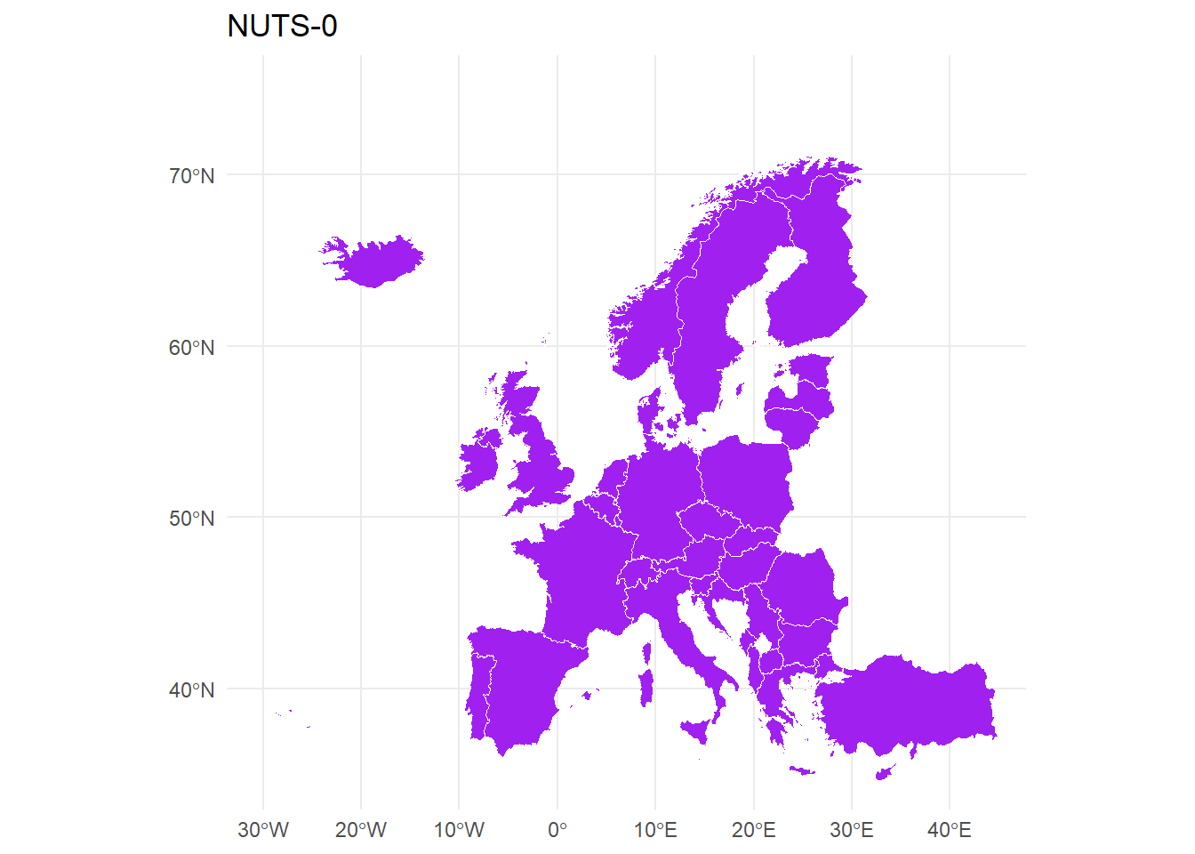
NUTS-1
# NUTS-1
mapdata_1 <- get_eurostat_geospatial(nuts_level = 1)
head(mapdata_1)
## Simple feature collection with 6 features and 7 fields
## geometry type:  MULTIPOLYGON
## dimension:      XY
## bbox:           xmin: 2.84672 ymin: 39.64579 xmax: 21.05607 ymax: 50.91189
## geographic CRS: WGS 84
##    id CNTR_CODE                                                   NUTS_NAME
## 1 AL0        AL                                                   SHQIPËRIA
## 2 AT1        AT                                               OSTÖSTERREICH
## 3 AT2        AT                                               SÜDÖSTERREICH
## 4 BE1        BE RÉGION DE BRUXELLES-CAPITALE/BRUSSELS HOOFDSTEDELIJK GEWEST
## 5 BE3        BE                                             RÉGION WALLONNE
## 6 AT3        AT                                              WESTÖSTERREICH
##   LEVL_CODE FID NUTS_ID                       geometry geo
## 1         1 AL0     AL0 MULTIPOLYGON (((19.831 42.4... AL0
## 2         1 AT1     AT1 MULTIPOLYGON (((15.54245 48... AT1
## 3         1 AT2     AT2 MULTIPOLYGON (((15.84791 47... AT2
## 4         1 BE1     BE1 MULTIPOLYGON (((4.47678 50.... BE1
## 5         1 BE3     BE3 MULTIPOLYGON (((5.682 50.75... BE3
## 6         1 AT3     AT3 MULTIPOLYGON (((14.69101 48... AT3

mapdata_1 %>%
  ggplot(., aes()) +
  geom_sf(fill="purple", color="white", size = 0.1) +
  theme_minimal() +
  xlim(c(-30, 44)) +
  ylim(c(35, 75)) +
  ggtitle("NUTS-1")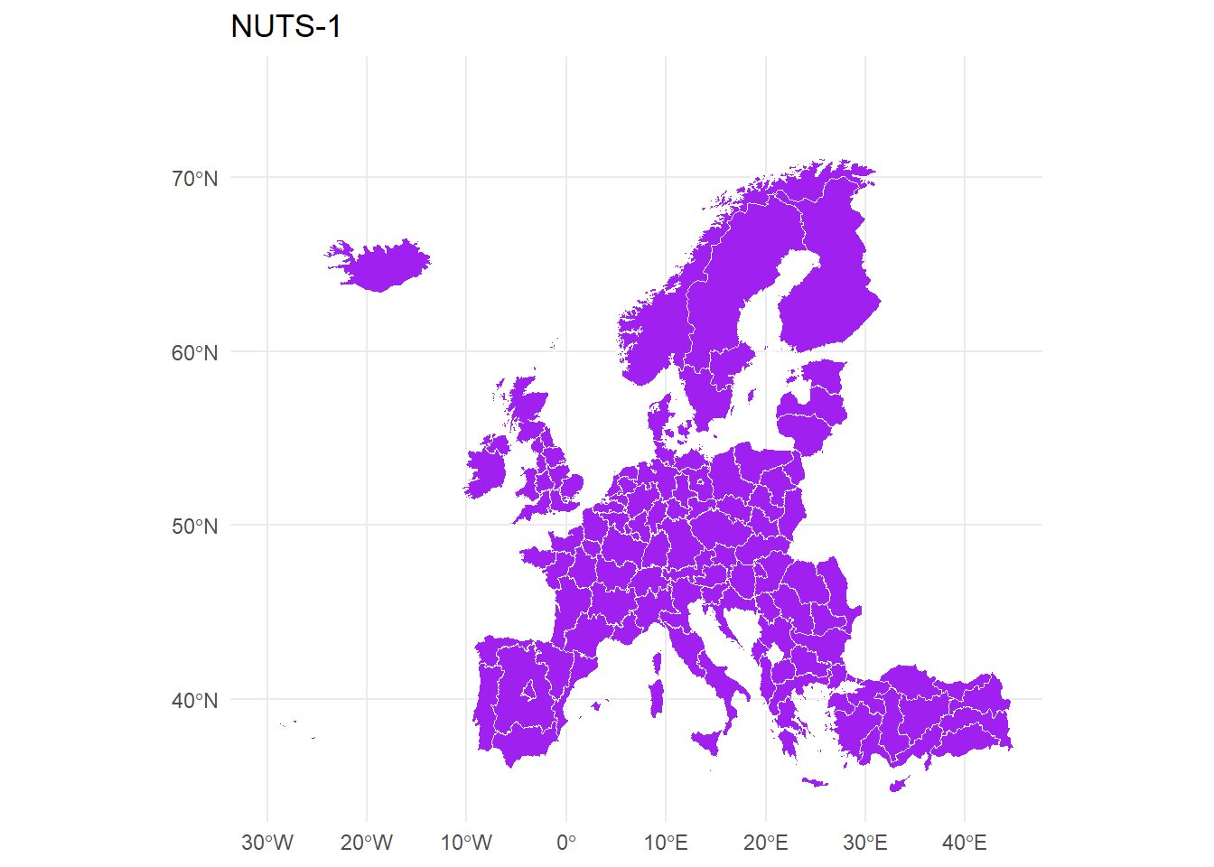
NUTS-2
# NUTS-2
mapdata_2 <- get_eurostat_geospatial(nuts_level = 2)
head(mapdata_2)
## Simple feature collection with 6 features and 7 fields
## geometry type:  MULTIPOLYGON
## dimension:      XY
## bbox:           xmin: 7.09629 ymin: 46.29368 xmax: 20.10688 ymax: 61.08726
## geographic CRS: WGS 84
##     id CNTR_CODE       NUTS_NAME LEVL_CODE  FID NUTS_ID
## 1 DE24        DE     Oberfranken         2 DE24    DE24
## 2 NO03        NO   Sør-Østlandet         2 NO03    NO03
## 3 HU11        HU        Budapest         2 HU11    HU11
## 4 HU12        HU            Pest         2 HU12    HU12
## 5 HU21        HU  Közép-Dunántúl         2 HU21    HU21
## 6 HU22        HU Nyugat-Dunántúl         2 HU22    HU22
##                         geometry  geo
## 1 MULTIPOLYGON (((11.48157 50... DE24
## 2 MULTIPOLYGON (((10.60072 60... NO03
## 3 MULTIPOLYGON (((18.93274 47... HU11
## 4 MULTIPOLYGON (((18.96591 47... HU12
## 5 MULTIPOLYGON (((18.68843 47... HU21
## 6 MULTIPOLYGON (((17.24743 48... HU22

mapdata_2 %>%
  ggplot(., aes()) +
  geom_sf(fill="purple", color="white", size = 0.1) +
  theme_minimal() +
  xlim(c(-30, 44)) +
  ylim(c(35, 75)) +
  ggtitle("NUTS-2")
NUTS-3
# NUTS-3
mapdata_3 <- get_eurostat_geospatial(nuts_level = 3)
head(mapdata_3)
## Simple feature collection with 6 features and 7 fields
## geometry type:  MULTIPOLYGON
## dimension:      XY
## bbox:           xmin: 2.3948 ymin: 39.02837 xmax: 22.2582 ymax: 60.65644
## geographic CRS: WGS 84
##      id CNTR_CODE
## 1 FRK23        FR
## 2 FRK24        FR
## 3 AT313        AT
## 4 FI200        FI
## 5 FR102        FR
## 6 EL611        EL
##                                                                   NUTS_NAME
## 1                                                                     Drôme
## 2                                                                     Isère
## 3                                                               Mühlviertel
## 4                                                                     Åland
## 5                                                           Seine-et-Marne
## 6 <U+039A>a<U+03C1>d<U+03AF>tsa, <U+03A4><U+03C1><U+03AF><U+03BA>a<U+03BB>a
##   LEVL_CODE   FID NUTS_ID                       geometry   geo
## 1         3 FRK23   FRK23 MULTIPOLYGON (((5.67604 44.... FRK23
## 2         3 FRK24   FRK24 MULTIPOLYGON (((5.10107 45.... FRK24
## 3         3 AT313   AT313 MULTIPOLYGON (((13.72709 48... AT313
## 4         3 FI200   FI200 MULTIPOLYGON (((19.94374 60... FI200
## 5         3 FR102   FR102 MULTIPOLYGON (((2.59053 49.... FR102
## 6         3 EL611   EL611 MULTIPOLYGON (((21.91769 39... EL611

mapdata_3 %>%
  ggplot(., aes()) +
  geom_sf(fill="purple", color="white", size = 0.1) +
  theme_minimal() +
  xlim(c(-30, 44)) +
  ylim(c(35, 75)) +
  ggtitle("NUTS-3")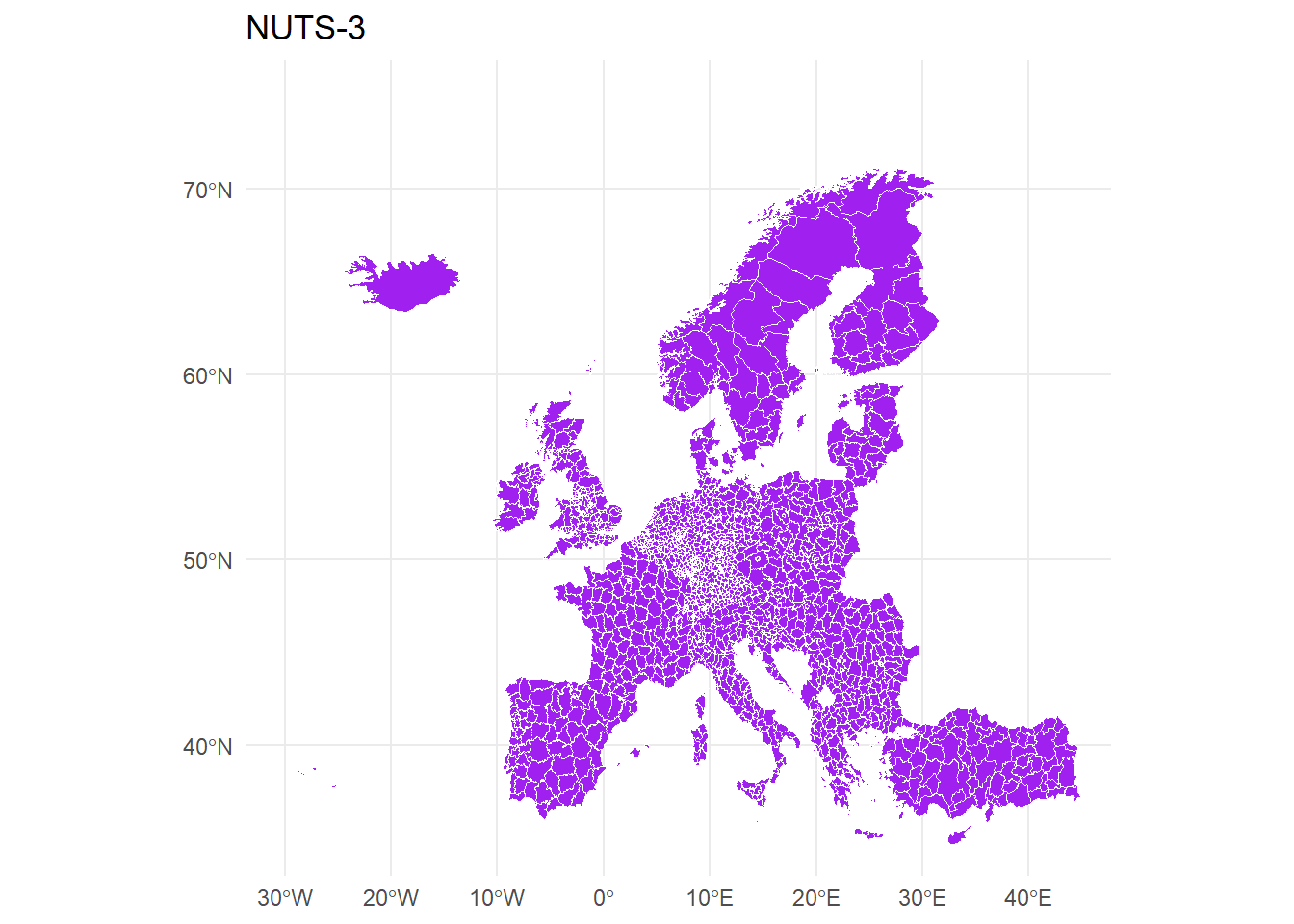
TODOS LOS NIVELES NUTS
# ALL NUTS
mapdata_all <- get_eurostat_geospatial(nuts_level = "all", resolution = 60)
head(mapdata_all)
## Simple feature collection with 6 features and 7 fields
## geometry type:  MULTIPOLYGON
## dimension:      XY
## bbox:           xmin: 2.54601 ymin: 34.56908 xmax: 34.56859 ymax: 51.50246
## geographic CRS: WGS 84
##   id CNTR_CODE                                                        NUTS_NAME
## 1 BG        BG <U+0411><U+042A><U+041B><U+0413><U+0410><U+0420><U+0418><U+042F>
## 2 CH        CH                                          SCHWEIZ/SUISSE/SVIZZERA
## 3 CY        CY                        <U+039A><U+03A5><U+03A0><U+03A1><U+039F>S
## 4 AL        AL                                                        SHQIPËRIA
## 5 CZ        CZ                                                  CESKÁ REPUBLIKA
## 6 BE        BE                                                 BELGIQUE-BELGIË
##   LEVL_CODE FID NUTS_ID                       geometry geo
## 1         0  BG      BG MULTIPOLYGON (((22.99717 43...  BG
## 2         0  CH      CH MULTIPOLYGON (((8.61383 47....  CH
## 3         0  CY      CY MULTIPOLYGON (((33.75237 34...  CY
## 4         0  AL      AL MULTIPOLYGON (((19.831 42.4...  AL
## 5         0  CZ      CZ MULTIPOLYGON (((14.49122 51...  CZ
## 6         0  BE      BE MULTIPOLYGON (((5.10218 51....  BE

mapdata_all %>%
  mutate(LEVL_CODE_2 = recode_factor(LEVL_CODE,
                                     `0`= "NUTS-0",
                                     `1`= "NUTS-1",
                                     `2`= "NUTS-2",
                                     `3`= "NUTS-3" )) %>%
  ggplot(., aes()) +
  geom_sf(fill="purple", color="white", size = 0.1) +
  theme_minimal() +
  xlim(c(-30, 44)) +
  ylim(c(35, 75)) +
  facet_wrap(~LEVL_CODE_2) +
  ggtitle("Unidades Territoriales Estadísticas (NUTS)")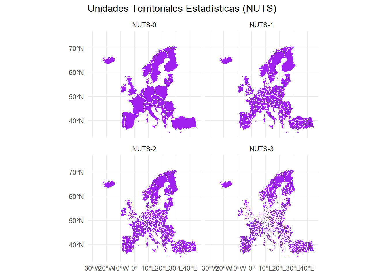
Spatial Polygon Dataframe (spdf)
En segundo lugar podemos descargar un Spatial Polygon Dataframe (spdf) utilizando el paquete {sf}, donde encontramos la información geográfica de todos los NUTS levels (0-3). De nuevo utilizamos la función get_eurostat_geospatial() y las funciones características de {tidyverse} y {ggplot2} para modificar el spdf y para seleccionar el nivel NUTS deseado.
# El Spatial Polygon Dataframe:

mapdata_spdf <- get_eurostat_geospatial(output_class = "spdf", resolution = 60)
NUTS-0
# NUTS 0

mapdata_spdf[mapdata_spdf$LEVL_CODE == 0,] %>%
  ggplot(., aes(x=long,y=lat,group=group)) +
  geom_polygon(fill="violetred4", color="white") +
  theme_minimal()+
  xlim(c(-30, 44)) +
  ylim(c(35, 75)) +
  ggtitle("NUTS-0")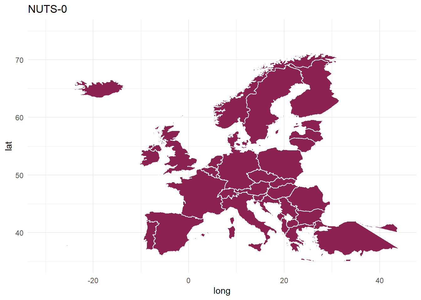
NUTS-1
# NUTS 1

mapdata_spdf[mapdata_spdf$LEVL_CODE == 1,] %>%
  ggplot(., aes(x=long,y=lat,group=group)) +
  geom_polygon(fill="violetred4", color="white") +
  theme_minimal()+
  xlim(c(-30, 44)) +
  ylim(c(35, 75)) +
  ggtitle("NUTS-1")
NUTS-2
# NUTS 2

mapdata_spdf[mapdata_spdf$LEVL_CODE == 2,] %>%
  ggplot(., aes(x=long,y=lat,group=group)) +
  geom_polygon(fill="violetred4", color="white") +
  theme_minimal()+
  xlim(c(-30, 44)) +
  ylim(c(35, 75))+
  ggtitle("NUTS-2")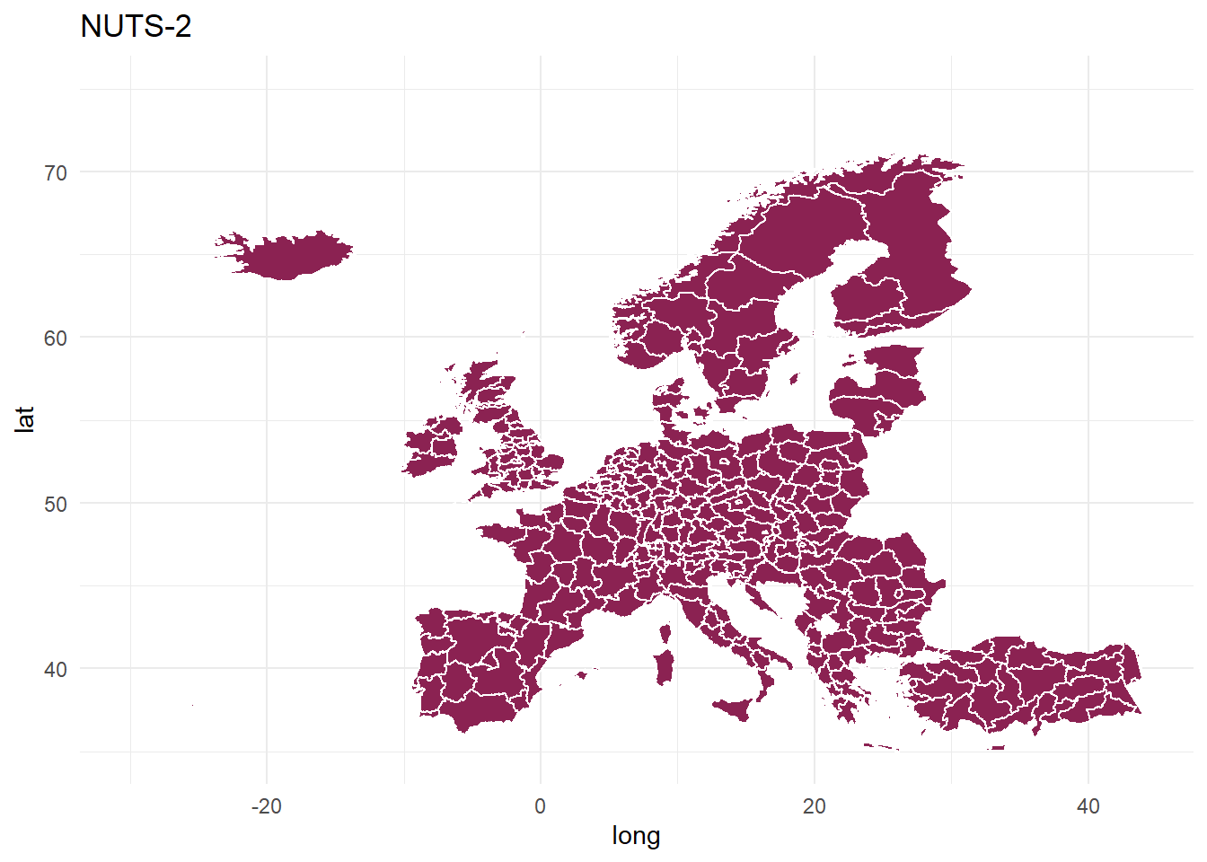
NUTS-3
# NUTS 3

mapdata_spdf[mapdata_spdf$LEVL_CODE == 3,] %>%
  ggplot(., aes(x=long,y=lat,group=group)) +
  geom_polygon(fill="violetred4", color="white") +
  theme_minimal()+
  xlim(c(-30, 44)) +
  ylim(c(35, 75))+
  ggtitle("NUTS-3")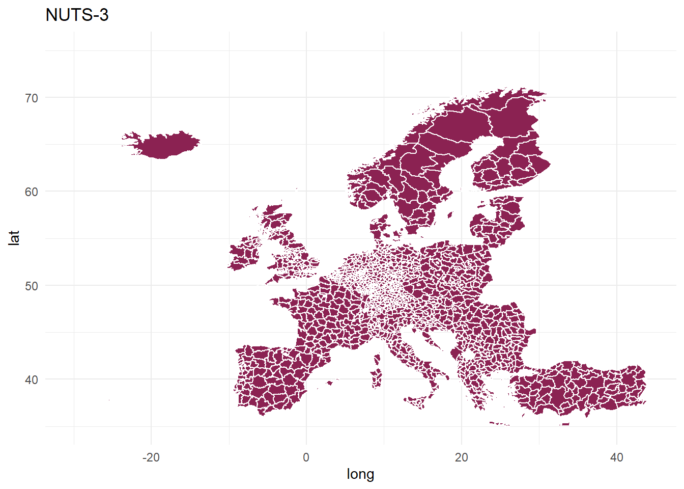
TODOS LOS NIVELES NUTS
Para representar los cuatro niveles de forma conjunta, y con la única intención de mostrar la funcionalidad de otro paquete de R, vamos a cambiar de procedimiento y utilizamos el paquete {cowflow} y su función plot_grid(). Para ello descargaremos los cuatro niveles NUTS por separado, guardamos cada uno de los gráficos de forma individualizada y utilizamos el paquete y la función mencionada para representar conjuntamente los cuatro gráficos.
mapdata_psdf_0 <- get_eurostat_geospatial(output_class = "spdf", nuts_level= 0, resolution = 60)
mapdata_psdf_1 <- get_eurostat_geospatial(output_class = "spdf", nuts_level= 1, resolution = 60)
mapdata_psdf_2 <- get_eurostat_geospatial(output_class = "spdf", nuts_level= 2, resolution = 60)
mapdata_psdf_3 <- get_eurostat_geospatial(output_class = "spdf", nuts_level= 3, resolution = 60)
nuts_0 <- mapdata_psdf_0 %>%
  ggplot(., aes(x=long,y=lat,group=group)) +
  geom_polygon(fill="tomato1", color="white", size = 0.1) +
  theme_minimal()+
  xlim(c(-30, 44)) +
  ylim(c(35, 75))

nuts_1 <- mapdata_psdf_1 %>%
  ggplot(., aes(x=long,y=lat,group=group)) +
  geom_polygon(fill="tomato2", color="white", size = 0.1) +
  theme_minimal()+
  xlim(c(-30, 44)) +
  ylim(c(35, 75))

nuts_2 <- mapdata_psdf_2 %>%
  ggplot(., aes(x=long,y=lat,group=group)) +
  geom_polygon(fill="tomato3", color="white", size = 0.1) +
  theme_minimal()+
  xlim(c(-30, 44)) +
  ylim(c(35, 75))

nuts_3 <- mapdata_psdf_3 %>%
  ggplot(., aes(x=long,y=lat,group=group)) +
  geom_polygon(fill="tomato4", color="white", size = 0.1) +
  theme_minimal()+
  xlim(c(-30, 44)) +
  ylim(c(35, 75))


plot_grid(nuts_0, nuts_1, nuts_2, nuts_3,
          labels= c("NUTS-0","NUTS-1","NUTS-2","NUTS-3"),
          label_size = 12)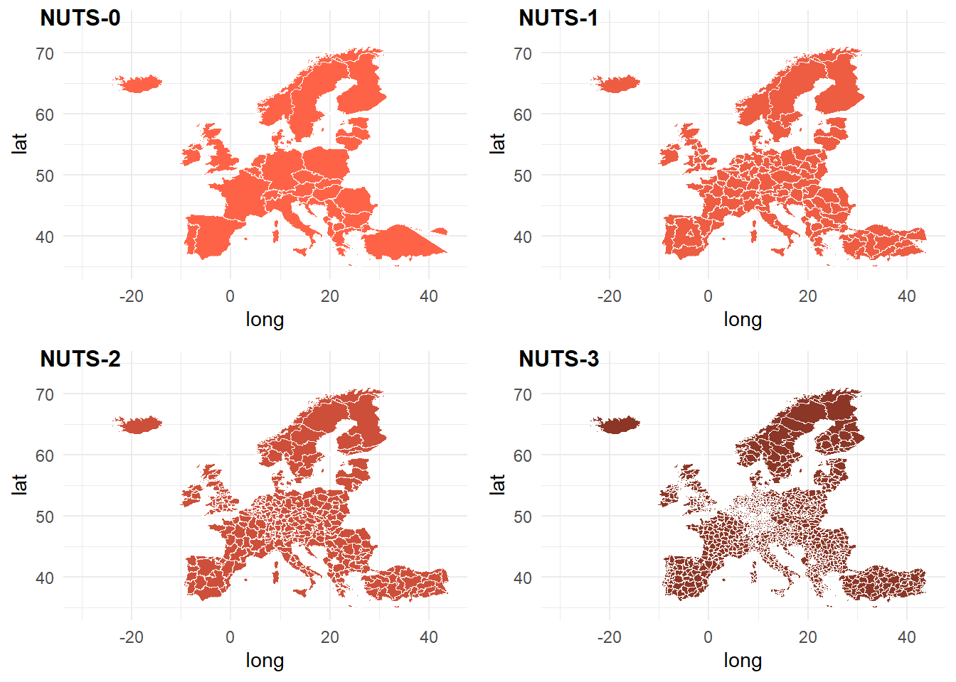
Dataframe (df)
Una tercera posibilidad consiste en descargar con la función get_eurostat_geospatial() un dataframe donde viene recopilada la información de todos los niveles de NUTS conjuntamente.
# Guardamos el dataframe con resolución 60

mapdata_df <- get_eurostat_geospatial(output_class = "df", resolution = 60)
head(mapdata_df)
## # A tibble: 6 x 13
##    long   lat order hole  piece group id    CNTR_CODE NUTS_NAME LEVL_CODE FID
##   <dbl> <dbl> <int> <lgl> <fct> <fct> <chr> <chr>     <chr>         <int> <chr>
## 1  23.0  43.8     1 FALSE 1     1.1   1     BG        <U+0411><U+042A><U+041B><U+0413><U+0410><U+0420><U+0418><U+042F>          0 BG
## 2  23.1  43.8     2 FALSE 1     1.1   1     BG        <U+0411><U+042A><U+041B><U+0413><U+0410><U+0420><U+0418><U+042F>          0 BG
## 3  23.1  43.8     3 FALSE 1     1.1   1     BG        <U+0411><U+042A><U+041B><U+0413><U+0410><U+0420><U+0418><U+042F>          0 BG
## 4  23.2  43.8     4 FALSE 1     1.1   1     BG        <U+0411><U+042A><U+041B><U+0413><U+0410><U+0420><U+0418><U+042F>          0 BG
## 5  23.3  43.8     5 FALSE 1     1.1   1     BG        <U+0411><U+042A><U+041B><U+0413><U+0410><U+0420><U+0418><U+042F>          0 BG
## 6  23.3  43.8     6 FALSE 1     1.1   1     BG        <U+0411><U+042A><U+041B><U+0413><U+0410><U+0420><U+0418><U+042F>          0 BG
## # ... with 2 more variables: NUTS_ID <chr>, geo <chr>
Podemos guardar un dataframe específico para cada nivel de NUTS. Utilizando el paquete {ggplot2} tal y como se ha utilizado en los ejemplos anteriores podemos realizar los diferentes mapas de Europa. En este caso, para evitar ser excesivamente repetitivos, únicamente vamos a representar el mapa conjunto utilizando la función facet_wrap().
# NUTS-0

mapdata_df_0 <- mapdata_df %>%
  filter(LEVL_CODE == 0)

# NUTS-1

mapdata_df_1 <- mapdata_df %>%
  filter(LEVL_CODE == 1)

# NUTS-2

mapdata_df_2 <- mapdata_df %>%
  filter(LEVL_CODE == 2)

# NUTS-3
mapdata_df_3 <- mapdata_df %>%
  filter(LEVL_CODE == 3)

# Usando la función facet_wrap() podemos visualizar los cuatro niveles de forma conjunta

mapdata_df %>%
  mutate(LEVL_CODE_2 = recode_factor(LEVL_CODE, `0`= "NUTS-0", `1`= "NUTS-1", `2`= "NUTS-2", `3`= "NUTS-3" )) %>%
  ggplot(., aes(x=long,y=lat, group=group)) +
  geom_polygon(fill="orange", color="white", size = 0.1) +
  theme_minimal() +
  xlim(c(-30, 44)) +
  ylim(c(35, 75)) +
  facet_wrap(~LEVL_CODE_2) +
  ggtitle("Unidades Territoriales Estadísticas (NUTS)")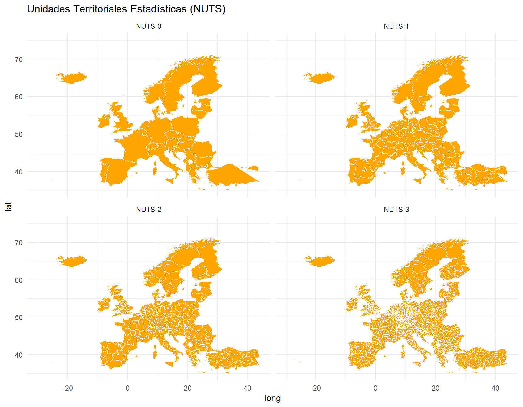
Mapas nacionales de las Unidades Territoriales Estadísticas (NUTS)
Podemos sustraer los códigos identificativos de cada país presentes en el dataframe utilizando la función unique() y, a partir de ahí, seleccionar los distintos niveles NUTS para examinar sus particularidades en los países de la Unión Europea. Veamos unos ejemplos examinando algunos países elegidos al azar:
unique(mapdata_df$CNTR_CODE)
##  [1] "BG" "CH" "CY" "AL" "CZ" "BE" "AT" "DE" "DK" "EE" "EL" "ES" "FI" "HR" "FR"
## [16] "HU" "IE" "IS" "IT" "LI" "LT" "LU" "LV" "ME" "MK" "MT" "NL" "NO" "PL" "PT"
## [31] "RO" "RS" "SE" "SI" "SK" "TR" "UK"
España
spain <- mapdata_df %>%
  mutate(LEVL_CODE_2 = recode_factor(LEVL_CODE,
                                     `0`= "NUTS-0",
                                     `1`= "NUTS-1",
                                     `2`= "NUTS-2",
                                     `3`= "NUTS-3" )) %>%
  filter(grepl("ES", NUTS_ID))


ggplot(spain, aes(x=long, y=lat, group=group)) +
  facet_wrap(~LEVL_CODE_2) +
  geom_polygon(fill="orange", color="white", size = 0.2) +
  theme_minimal() +
  ggtitle("España")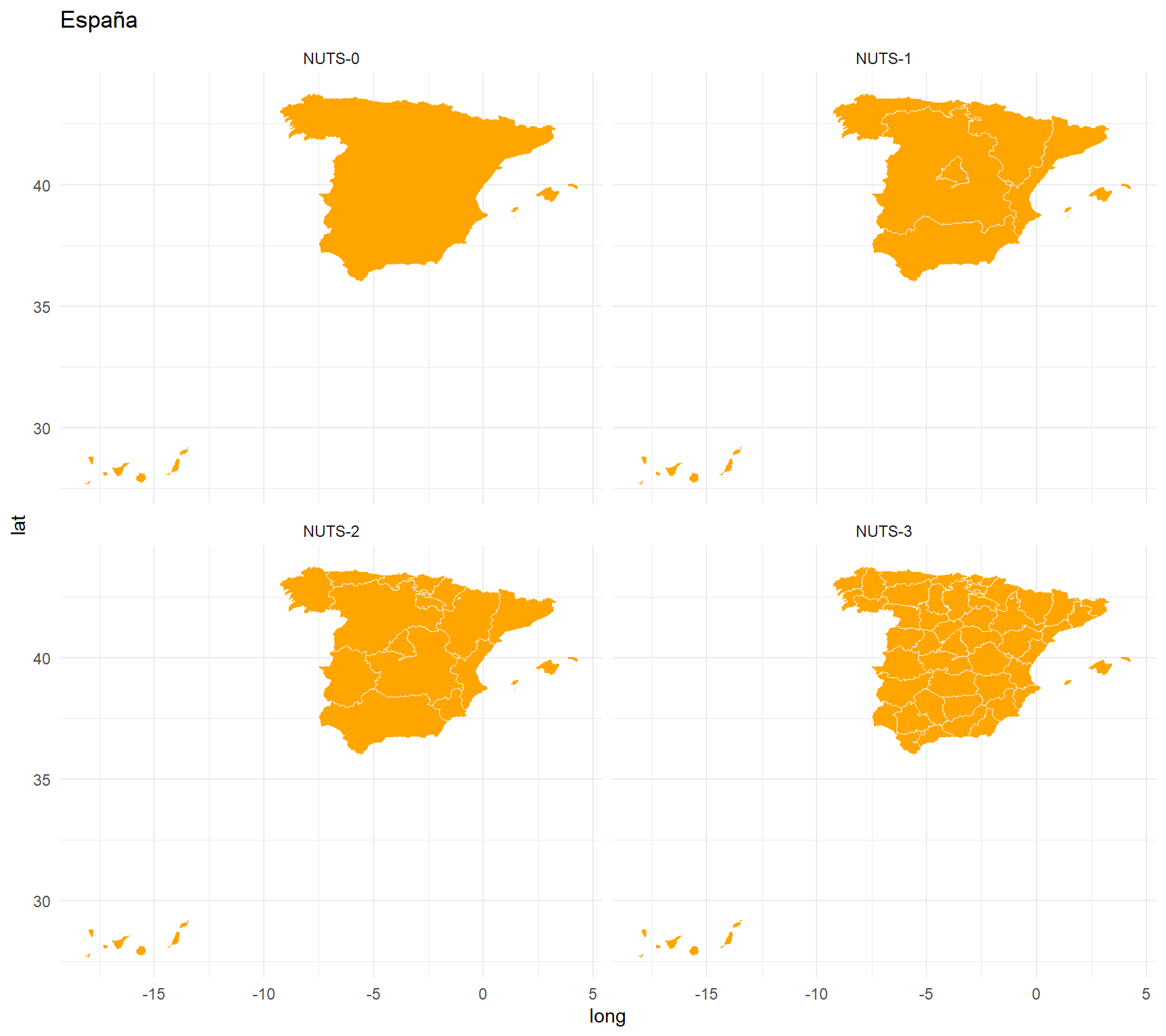
Italia
italy <- mapdata_df %>%
  mutate(LEVL_CODE_2 = recode_factor(LEVL_CODE,
                                     `0`= "NUTS-0",
                                     `1`= "NUTS-1",
                                     `2`= "NUTS-2",
                                     `3`= "NUTS-3" )) %>%
  filter(grepl("IT", NUTS_ID))


ggplot(italy, aes(x=long, y=lat, group=group)) +
  facet_wrap(~LEVL_CODE_2) +
  geom_polygon(fill="orange", color="white", size = 0.2) +
  theme_minimal()+
  ggtitle("Italia")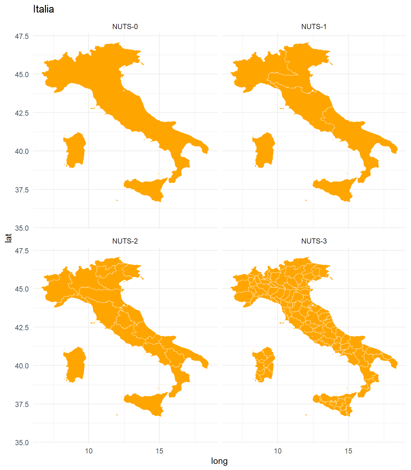
Francia
france <- mapdata_df %>%
  mutate(LEVL_CODE_2 = recode_factor(LEVL_CODE,
                                     `0`= "NUTS-0",
                                     `1`= "NUTS-1",
                                     `2`= "NUTS-2",
                                     `3`= "NUTS-3" )) %>%
  filter(grepl("FR", NUTS_ID))


ggplot(france, aes(x=long, y=lat, group=group)) +
  facet_wrap(~LEVL_CODE_2) +
  geom_polygon(fill="orange", color="white", size = 0.2) +
  xlim(c(-8, 12)) +
  ylim(c(40, 53)) +
  theme_minimal()+
  ggtitle("Francia")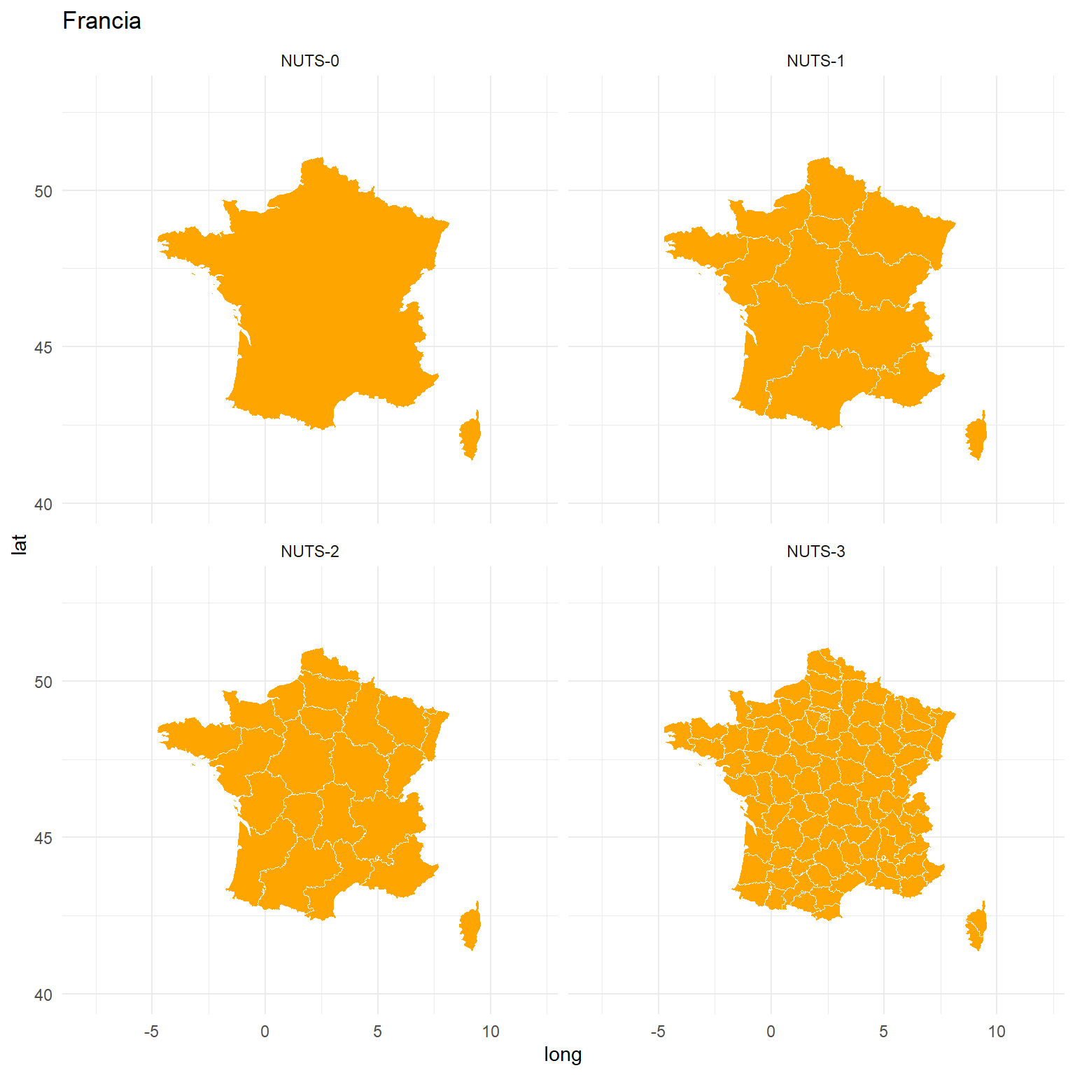
Alemania
germany <- mapdata_df %>%
  mutate(LEVL_CODE_2 = recode_factor(LEVL_CODE,
                                     `0`= "NUTS-0",
                                     `1`= "NUTS-1",
                                     `2`= "NUTS-2",
                                     `3`= "NUTS-3" )) %>%
  filter(grepl("DE", NUTS_ID))


ggplot(germany, aes(x=long, y=lat, group=group)) +
  facet_wrap(~LEVL_CODE_2) +
  geom_polygon(fill="orange", color="white", size = 0.2) +
  theme_minimal()+
  ggtitle("Alemania")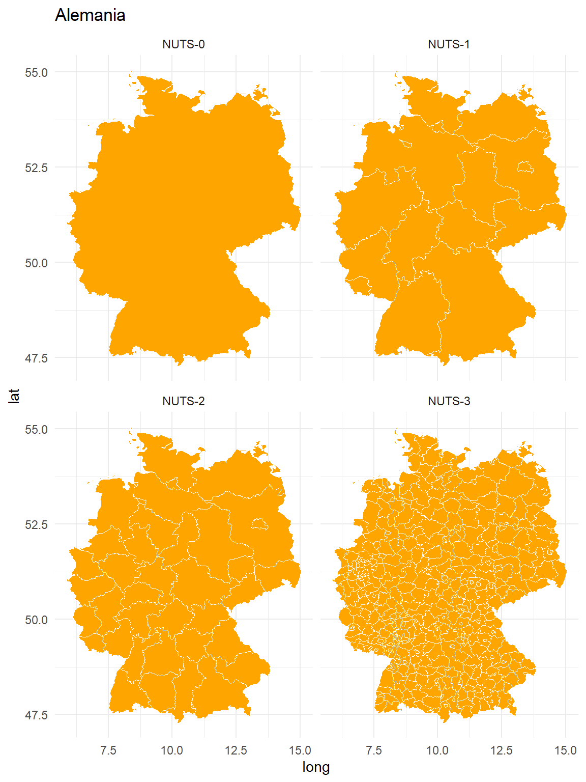
Reino Unido
unitedkingdom <- mapdata_df %>%
  mutate(LEVL_CODE_2 = recode_factor(LEVL_CODE,
                                     `0`= "NUTS-0",
                                     `1`= "NUTS-1",
                                     `2`= "NUTS-2",
                                     `3`= "NUTS-3" )) %>%
  filter(grepl("UK", NUTS_ID))


ggplot(unitedkingdom, aes(x = long, y=lat, group = group)) +
  facet_wrap(~LEVL_CODE_2) +
  geom_polygon(fill="orange", color="white", size = 0.2) +
  theme_minimal()+
  ggtitle("Reino Unido")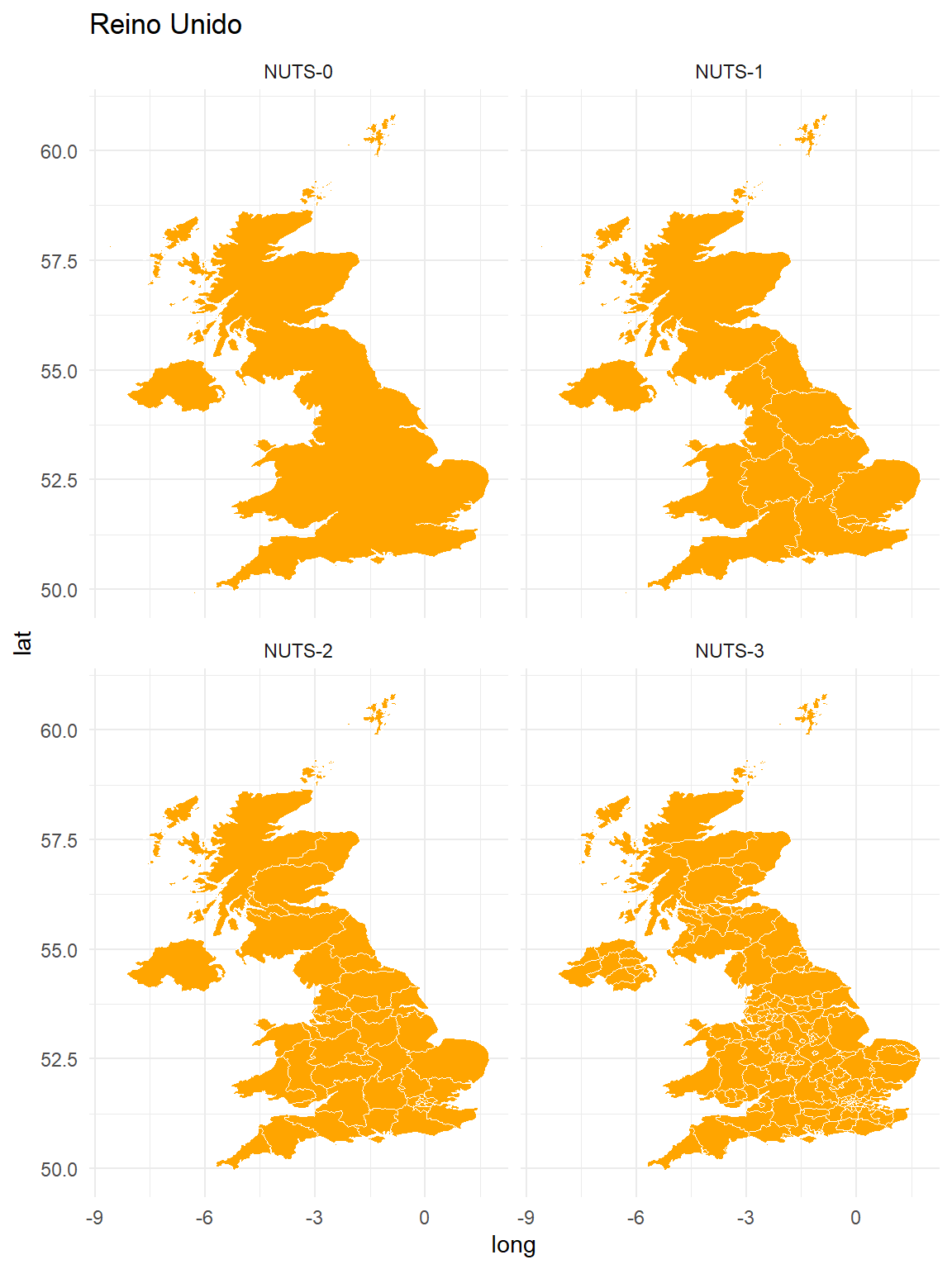
Aplicación práctica utilizando datos de Eurostat
NUTS-0. Ratio de Mortalidad Infantil
En primer lugar vamos a representar en un mapa el ratio de mortalidad infantil en el año 2017 por países (NUTS 0). En Eurostat este ratio (infant mortality rate) indica el número de muertes de bebés menores de 1 año por cada mil nacimientos. Para ello, lo primero que hacemos es buscar en la base de datos de Eurostat indicando la palabra “mortality” y, una vez seleccionado el dataframe que nos interesa, lo descargamos y guardamos como inf_mort_rate.
# Buscamos el dataset

mortality <- search_eurostat(pattern = "mortality",
                                type = "table")

mortality %>%
  select(title, code)
## # A tibble: 4 x 2
##   title                                                                 code
##   <chr>                                                                 <chr>
## 1 Infant mortality rate                                                 tps00027
## 2 Standardised preventable and treatable mortality                      sdg_03_~
## 3 Standardised preventable and treatable mortality                      sdg_03_~
## 4 Assessed fish stocks exceeding fishing mortality at maximum sustaina~ sdg_14_~


# Descargamos el dataset "Infant mortality rate" utilizando el id (tps00027)

inf_mort_rate <- get_eurostat(id= "tps00027",  time_format = "num")

head(inf_mort_rate)
## # A tibble: 6 x 5
##   unit  indic_de geo    time values
##   <fct> <fct>    <fct> <dbl>  <dbl>
## 1 RT    INFMORRT AD     2007    2.4
## 2 RT    INFMORRT AL     2007    6.2
## 3 RT    INFMORRT AM     2007   10.8
## 4 RT    INFMORRT AT     2007    3.7
## 5 RT    INFMORRT AZ     2007   11.6
## 6 RT    INFMORRT BA     2007    6.8
Los códigos que identifican los países incluidos en el mapa base previamente realizado son los siguientes:
country_codes <- unique(mapdata_0$NUTS_ID)
country_codes
##  [1] "BG" "CH" "CY" "AL" "CZ" "BE" "AT" "DE" "DK" "EE" "EL" "ES" "FI" "HR" "FR"
## [16] "HU" "IE" "IS" "IT" "LI" "LT" "LU" "LV" "ME" "MK" "MT" "NL" "NO" "PL" "PT"
## [31] "RO" "RS" "SE" "SI" "SK" "TR" "UK"
Realizamos una serie de modificaciones al dataframe inf_mort_rate para seleccionar el año 2017 e identificar las regiones que debemos incluir en nuestro mapa.
inf_mort_2017 <- inf_mort_rate %>%
  filter( time == "2017") %>%
  filter(geo %in% country_codes )
Unimos los dos dataframes en uno que denominamos inf_mort_2017_mapa y seleccionamos el número de rangos en los que queremos clasificar los ratios de mortalidad infantil (en este caso determinamos 10 categorías).
inf_mort_2017_mapa <- mapdata_0 %>%
  right_join(inf_mort_2017) %>%
  mutate(cat = cut_to_classes(values, n=10, decimals = 1))
Y finalmente graficamos:
ggplot(inf_mort_2017_mapa, aes(fill=cat)) +
  geom_sf(color = alpha("white", 1/2), alpha= .9) +
  xlim(c(-20, 44)) +
  ylim(c(35, 70)) +
  labs(title = "Ratio de Mortalidad Infantil (%), 2017",
       subtitle = "Núm de muertes infantiles (menores de 1 año) por cada mil nacidos vivos",
       caption = "Fuente: Eurostat",
       fill= "") +
  theme_minimal() +
  theme(
    axis.line = element_blank(),
    axis.text = element_blank(),
    axis.title = element_blank(),
    axis.ticks = element_blank(),
    plot.background = element_rect(fill = "snow", color = NA),
    panel.background = element_rect(fill= "snow", color = NA),
    plot.title = element_text(size = 16, hjust = 0.5),
    plot.subtitle = element_text(size = 10, hjust = 0.5),
    plot.caption = element_text(size = 8, hjust = 1),
    legend.title = element_text(color = "grey40", size = 8),
    legend.text = element_text(color = "grey40", size = 7, hjust = 0),
    legend.position = c(0.93, 0.6),
    plot.margin = unit(c(0.5,2,0.5,1), "cm")) +
  scale_fill_brewer(palette= "Spectral")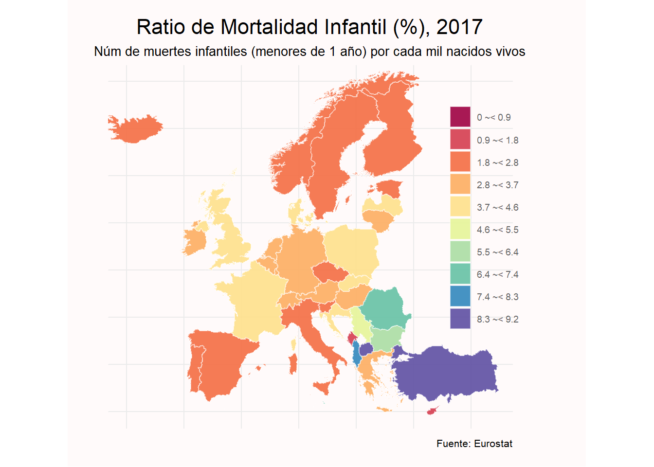
NUTS-2. Jóvenes que ni estudian ni trabajan
En el segundo ejemplo vamos a tratar de representar en un mapa de Europa (NUTS-2) el ratio de jóvenes que no se encuentraban trabajando ni cursando algún tipo de formación en el año 2016. Eurostat denomina a este ratio como el NEET rate (Youth not in employment, education or training).
De nuevo buscamos y descargamos la información directamente de Eurostat al igual que hicimos en el ejemplo anterior. En este caso el id que vamos a utilizar es edat_lfse_22.
neet <- get_eurostat(id= "edat_lfse_22",  time_format = "num")

neet_label <- label_eurostat(neet, fix_duplicated = T)
Conviene examinar las variables del dataframe y las categorías que comprende dicho dataframe:
label_eurostat_vars(names(neet))
## [1] "Sex"                             "Age class"
## [3] "Training"                        "Activity and employment status"
## [5] "Unit of measure"                 "Geopolitical entity (reporting)"
## [7] "Period of time"
levels(neet$sex)
## [1] "F" "M" "T"
levels(neet$age)
## [1] "Y15-24" "Y18-24"
levels(neet$training)
## [1] "NO_FE_NO_NFE"
levels(neet$wstatus)
## [1] "NEMP"
levels(neet$unit)
## [1] "PC"
Seleccionamos los códigos regionales del mapa base que mostramos en apartados previos con el objetivo de, posteriormente, seleccionar dichos valores del dataset neet obtenido de Eurostat.
regions_codes <- unique(mapdata_df_2$geo)
Posteriormente realizamos algunas modificaciones sobre el dataset para identificar el año, ambos sexos y el rango de edad que vamos a tener en consideración: 15-24 años. Además, seleccionamos los valores que se corresponden a las regiones presentes en el mapa base utilizando los códigos identificados previamente.
neet_total_2016 <- neet %>%
  filter(sex == "T",
         age == "Y15-24",
         time == 2016,
         geo %in% regions_codes) %>%
  select(geo, values)
Unimos los dataset y aplicamos un conjunto de rangos atendiendo a los valores. En este caso identificamos de nuevo 10 rangos para su posterior representación gráfica.
neet_total_map <- mapdata_df_2 %>%
  right_join(neet_total_2016) %>%
  mutate(cat = cut_to_classes(values, n=10, decimals=1))
Utilizamos básicamente los colores de la paleta denominada “Spectral”. No obstante, sobre los colores de dicha paleta realizamos alguna sencilla modificación con el objetivo de incluir en nuestra selección un color gris para indicar las regiones europeas donde no tenemos información disponible.
La función brewer.pal() del paquete RColorBrewer nos permite identificar los colores que componen la paleta en questión y la función display.brewer.pal() nos permite visualizar dichos colores. De esta forma podemos identificar los colores que queremos conservar y los colores que nos interesa añadir en nuestra selección de colores final.
brewer.pal(11, "Spectral")
##  [1] "#9E0142" "#D53E4F" "#F46D43" "#FDAE61" "#FEE08B" "#FFFFBF" "#E6F598"
##  [8] "#ABDDA4" "#66C2A5" "#3288BD" "#5E4FA2"
display.brewer.pal(11, "Spectral")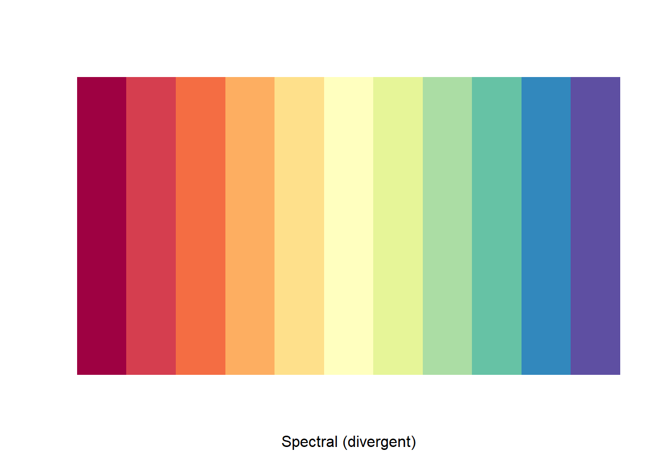
colores <- c("grey60", "#5E4FA2", "#3288BD", "#66C2A5", "#ABDDA4", "#FFFFBF", "#FEE08B","#FDAE61", "#F46D43","#D53E4F", "#9E0142")
Y graficamos indicando los colores seleccionados con la función scale_fill_manual().
ggplot(neet_total_map, aes(x= long, y=lat, group= group)) +
  geom_polygon(aes(fill = cat),
               color = "white",
               alpha= .9,
               size = 0.05) +
  xlim(c(-24, 44)) +
  ylim(c(35, 72)) +
  labs(title = "Young people (15-24 Yrs) neither in employment nor in education/training \n(NEET rate in 2016)",
       subtitle = "NUTS-2 regions",
       caption = "Fuente: Eurostat",
       fill= "") +
  theme_minimal() +
  theme(
    axis.line = element_blank(),
    axis.text = element_blank(),
    axis.title = element_blank(),
    axis.ticks = element_blank(),
    plot.background = element_rect(fill = "snow", color = NA),
    panel.background = element_rect(fill= "snow", color = NA),
    plot.title = element_text(size = 13, hjust = 0.5),
    plot.subtitle = element_text(size = 10, hjust = 0.5),
    plot.caption = element_text(size = 8, hjust = 1),
    legend.title = element_text(color = "grey40", size = 8),
    legend.text = element_text(color = "grey40", size = 7, hjust = 0),
    legend.position = c(0.93, 0.6),
    plot.margin = unit(c(0.5,2,0.5,1), "cm")) +
  scale_fill_manual(values= colores)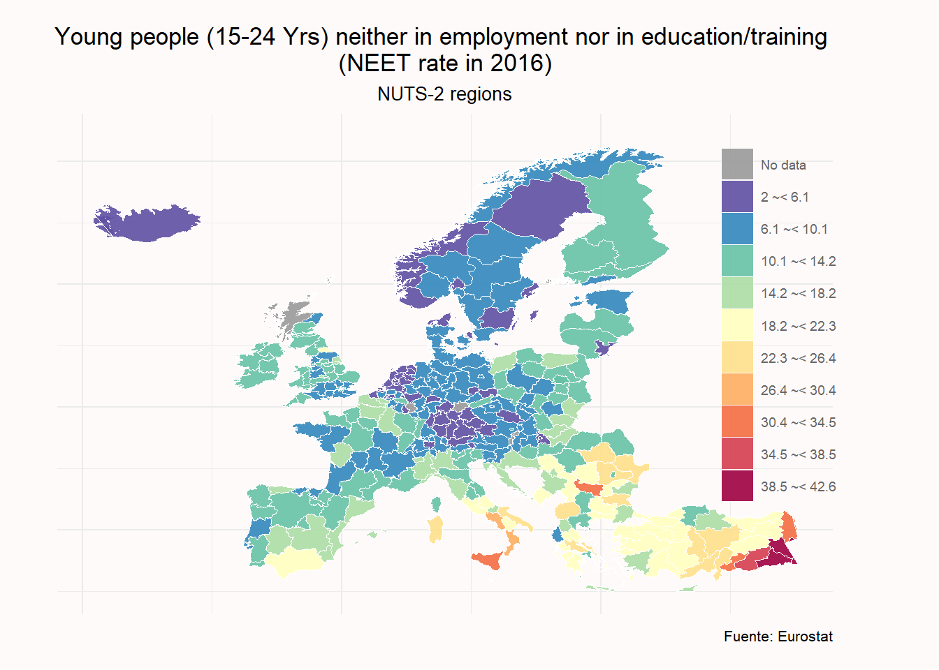
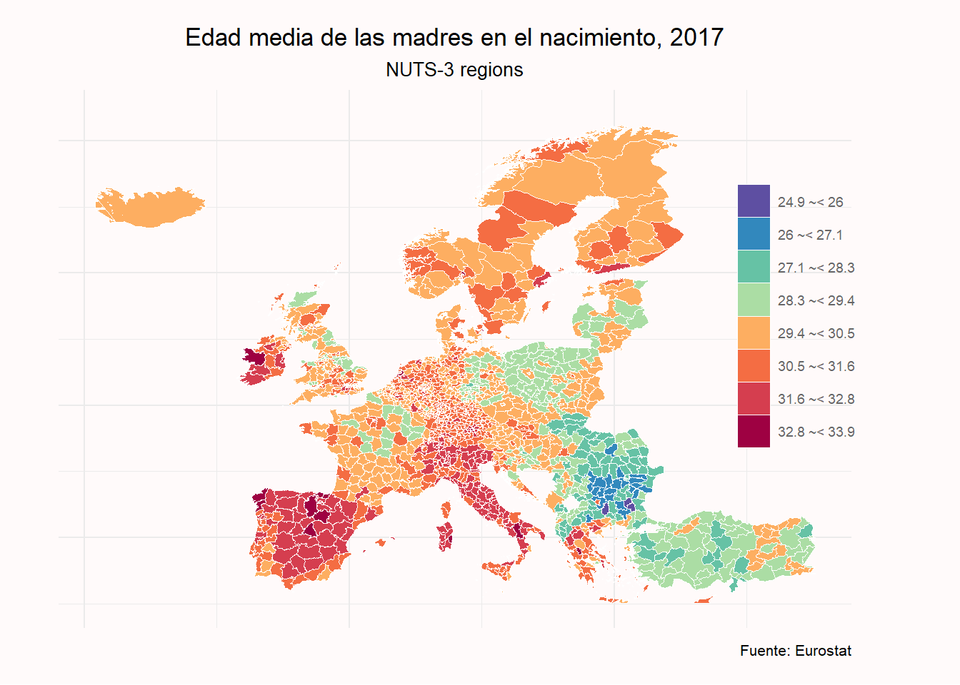
NUTS-3. Edad promedio de las madres en el nacimiento
Para terminar vamos a exponer un ejemplo de mapa a nivel NUT-3. En esta ocasión vamos a representar gráficamente la edad promedio (media) de las madres en los nacimientos. Para ello seguimos un procedimiento similar al seguido en el apartado anterior.
En primer lugar buscamos y descargamos la información que se ajusta a nuestro interés.
fertility <- get_eurostat(id= "demo_r_find3",  time_format = "num")
fertility_label <- label_eurostat(fertility, fix_duplicated = T)
Examinamos las variables del dataset y las categorías en las que se estructura el mismo.
label_eurostat_vars(names(fertility))
## [1] "Demographic indicator"           "Unit of measure"
## [3] "Geopolitical entity (reporting)" "Period of time"
levels(fertility$indic_de)
## [1] "AGEMOTH"    "MEDAGEMOTH" "TOTFERRT"
levels(fertility_label$indic_de)
## [1] "Mean age of women at childbirth"   "Median age of women at childbirth"
## [3] "Total fertility rate"
Seleccionamos el código de las regiones en función al mapa base realizado previamente.
regions_3_codes <- unique(mapdata_df_3$geo)
Manipulamos el dataframe para seleccionar únicamente el año de interés, en este caso el año 2017, y la categoría que nos interesa: la edad media de las madres.
fertility_total_2017 <- fertility %>%
  filter(time == 2017,
         indic_de == "AGEMOTH",
         geo %in% regions_3_codes) %>%
  select(geo, values)
Unimos los datasets en uno que nos servirá para realizar nuestro mapa final.
fertility_total_map <- mapdata_df_3 %>%
  right_join(fertility_total_2017) %>%
  mutate(cat = cut_to_classes(values, n=8, decimals=1))
Seleccionamos los colores que vamos a utilizar para los rangos de valores. En este caso hemos establecido 8 rangos y, consecuentemente, seleccionamos 8 colores.
colores_2 <- c("#5E4FA2", "#3288BD", "#66C2A5", "#ABDDA4","#FDAE61", "#F46D43","#D53E4F", "#9E0142")
Realizamos el gráfico final
ggplot(fertility_total_map, aes(x= long, y=lat, group= group)) +
  geom_polygon(aes(fill = cat),
               color = "white",
               size = 0.005) +
  xlim(c(-24, 44)) +
  ylim(c(35, 72)) +
  labs(title = "Edad media de las madres en el nacimiento, 2017",
       subtitle = "NUTS-3 regions",
       caption = "Fuente: Eurostat",
       fill= "") +
  theme_minimal() +
  theme(
    axis.line = element_blank(),
    axis.text = element_blank(),
    axis.title = element_blank(),
    axis.ticks = element_blank(),
    plot.background = element_rect(fill = "snow", color = NA),
    panel.background = element_rect(fill= "snow", color = NA),
    plot.title = element_text(size = 13, hjust = 0.5),
    plot.subtitle = element_text(size = 10, hjust = 0.5),
    plot.caption = element_text(size = 8, hjust = 1),
    legend.title = element_text(color = "grey40", size = 8),
    legend.text = element_text(color = "grey40", size = 7, hjust = 0),
    legend.position = c(0.93, 0.6),
    plot.margin = unit(c(0.5,2,0.5,1), "cm")) +
  scale_fill_manual(values= colores_2)