Carreteras

Pongamos que nos interesa representar gráficamente la red de carreteras de Zaragoza. En este caso identificaremos highway como key y seleccionaremos un conjunto de valores obtenidos previamente:

carreteras <- getbb("Zaragoza Spain")%>%
  opq()%>%
  add_osm_feature(key = "highway", 
                  value = c("road", "motorway", "primary", 
                            "secondary", "tertiary")) %>%
  osmdata_sf()


carreteras
## Object of class 'osmdata' with:
##                  $bbox : 41.4516625,-1.1737289,41.9314873,-0.6803895
##         $overpass_call : The call submitted to the overpass API
##                  $meta : metadata including timestamp and version numbers
##            $osm_points : 'sf' Simple Features Collection with 22630 points
##             $osm_lines : 'sf' Simple Features Collection with 3095 linestrings
##          $osm_polygons : 'sf' Simple Features Collection with 49 polygons
##        $osm_multilines : NULL
##     $osm_multipolygons : NULL

Una vez hemos indicado los elementos que nos interesa representar en el mapa, en nuestro caso carreteras, procedemos a graficar utilizando {ggplot2}.

ggplot() +
  geom_sf(data = carreteras$osm_lines,
          inherit.aes = FALSE,
          color = "darkgrey",
          size = .4,
          alpha = .8)+
  labs(title = "Zaragoza",
       subtitle = "Red de carreteras")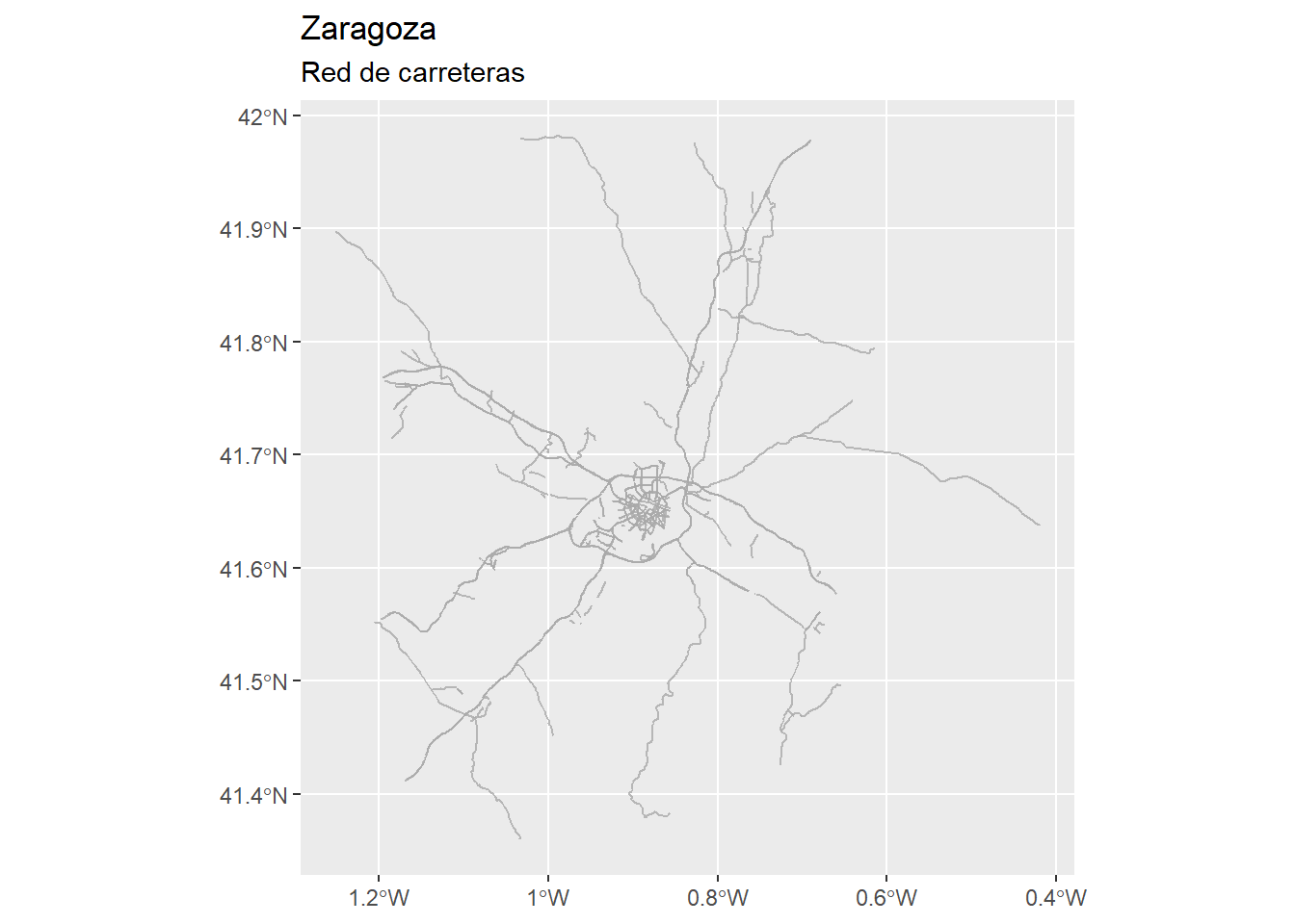

El gráfico anterior utiliza las coordenadas obtenidas mediante la función getbb(). De esta forma las coordenadas utilizadas al realizar el mapa anterior han sido las siguientes:

getbb("Zaragoza Spain")
##         min        max
## x -1.173729 -0.6803895
## y 41.451662 41.9314873

No obstante podemos modificar fácilmente dichas coordenadas geográficas. Supongamos, por ejemplo, que nos interesa realizar un mapa de las carreteras de la ciudad de Zaragoza y, a lo sumo, de su perímetro cercano. Una posibilidad sería indicar las coordinadas deseadas con coord_sf de la siguiente forma:

ggplot() +
  geom_sf(data = carreteras$osm_lines,
          inherit.aes = FALSE,
          color = "darkgrey",
          size = .4,
          alpha = .8)+
  coord_sf(xlim = c(-0.98, -0.8), 
           ylim = c(41.6, 41.7),
           expand = FALSE) +
  theme_void() +
  labs(title = "Zaragoza",
       subtitle = "Red de carreteras")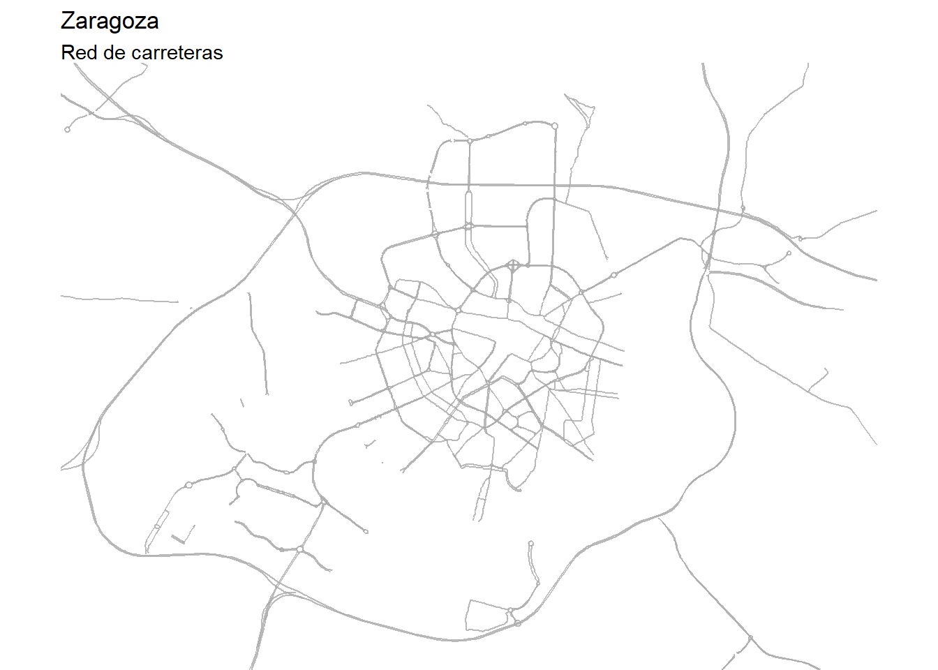

Alternativamente podemos indicar las coordenadas geográficas de nuestro mapa de la siguiente forma:

min <- c(-0.95, 41.6)
max <- c(-0.8, 41.7)
zgz_df <- as.matrix(data.frame(min, max))
row.names(zgz_df) <- c("x","y")

carreteras_B <- zgz_df%>%
  opq()%>%
  add_osm_feature(key = "highway", 
                  value = c("road", "motorway", "primary", 
                            "secondary", "tertiary")) %>%
  osmdata_sf()

carreteras_B
## Object of class 'osmdata' with:
##                  $bbox : 41.6,-0.95,41.7,-0.8
##         $overpass_call : The call submitted to the overpass API
##                  $meta : metadata including timestamp and version numbers
##            $osm_points : 'sf' Simple Features Collection with 12728 points
##             $osm_lines : 'sf' Simple Features Collection with 2224 linestrings
##          $osm_polygons : 'sf' Simple Features Collection with 11 polygons
##        $osm_multilines : NULL
##     $osm_multipolygons : NULL

El mapa resultante será, evidentemente, similar al obtenido previamente.

ggplot() +
  geom_sf(data = carreteras_B$osm_lines,
          inherit.aes = FALSE,
          color = "darkgrey",
          size = .4,
          alpha = .8) +
  theme_void() +
  labs(title = "Zaragoza",
       subtitle = "Red de carreteras")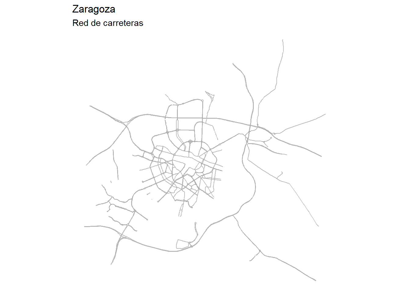

Calles

Me resulta difícil identificar mi ciudad observando únicamente su red de carreteras. Por ello vamos a representar en el mapa las calles que conforman la ciudad. Para ello utilizaremos algunas de la subcategorías de las mostradas previamente dentro de la categoría “highway”.

calles <- getbb("Zaragoza Spain")%>%
  opq()%>%
  add_osm_feature(key = "highway", 
                  value = c("residential", "living_street",
                            "unclassified",
                            "service", "footway")) %>%
  osmdata_sf()

ggplot() +
  geom_sf(data = calles$osm_lines,
          inherit.aes = FALSE,
          color = "darkgrey",
          size = .3,
          alpha = .8)+
  coord_sf(xlim = c(-0.98, -0.8), 
           ylim = c(41.6, 41.7),
           expand = FALSE) +
  theme_void() +
  labs(title = "Zaragoza")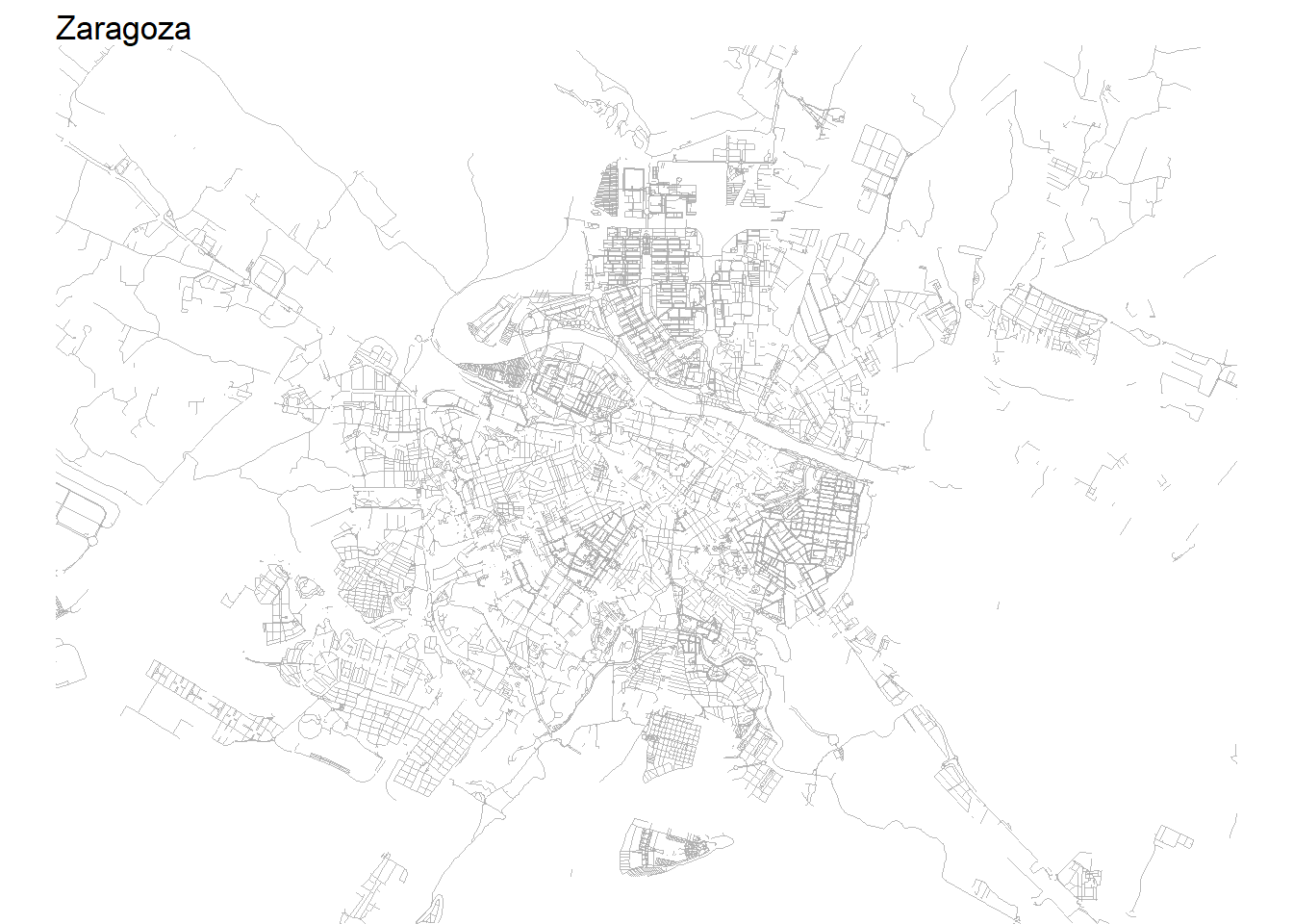

Esto ya me resulta más familiar. Representemos ahora, en el mismo mapa, las calles y la red de carreteras del mapa anterior.

ggplot() +
  geom_sf(data = calles$osm_lines,
          inherit.aes = FALSE,
          color = "darkgrey",
          size = .2,
          alpha = .8)+
  geom_sf(data = carreteras$osm_lines,
          inherit.aes = FALSE,
          color = "black",
          size = .2,
          alpha = .8)+
  coord_sf(xlim = c(-0.98, -0.8), 
           ylim = c(41.6, 41.7),
           expand = FALSE) +
  theme_void() +
  labs(title = "Zaragoza")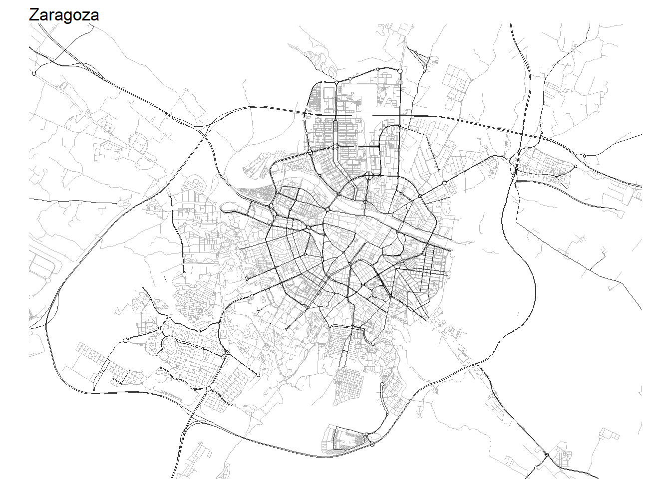

Ríos

Zaragoza, sin Ebro, no es Zaragoza. Veamos cómo hacer para representar los ríos y, ya puestos, los canales.

rios <- getbb("Zaragoza Spain")%>%
  opq()%>%
  add_osm_feature(key = "waterway", 
                  value = c("river", "canal")) %>%
  osmdata_sf()
  

Graficamos los ríos (Ebro, Huerva y Gállego) y los diversos canales que fluyen en la ciudad:

ggplot() +
  geom_sf(data = calles$osm_lines,
          inherit.aes = FALSE,
          color = "darkgrey",
          size = .2,
          alpha = .8)+
  geom_sf(data = carreteras$osm_lines,
          inherit.aes = FALSE,
          color = "black",
          size = .2,
          alpha = .8)+
  geom_sf(data = rios$osm_lines,
          inherit.aes = FALSE,
          color = "#7fc0ff",
          size = .8,
          alpha = .8) +
  coord_sf(xlim = c(-0.98, -0.8), 
           ylim = c(41.6, 41.7),
           expand = FALSE) +
  theme_void() +
  labs(title = "Zaragoza")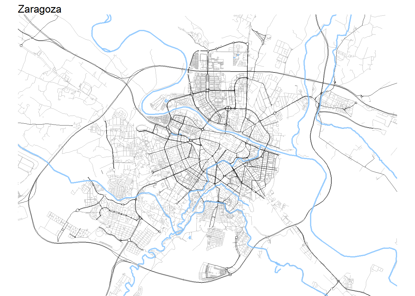

Es posible realizar modificaciones de algún elemento visual sobre el mapa previo. Pongamos, por ejemplo, que nos atrae más un fondo oscuro para nuestro mapa y queremos representar las calles de un color más vistoso o llamativo. Una posibilidad sería realizar las siguientes operaciones:

ggplot() +
  geom_sf(data = calles$osm_lines,
          inherit.aes = FALSE,
          color = "orange",
          size = .1,
          alpha = .8)+
  geom_sf(data = carreteras$osm_lines,
          inherit.aes = FALSE,
          color = "grey40",
          size = .2,
          alpha = .8)+
  geom_sf(data = rios$osm_lines,
          inherit.aes = FALSE,
          color = "white",
          size = .5,
          alpha = .8) +
  coord_sf(xlim = c(-0.98, -0.8), 
           ylim = c(41.6, 41.7),
           expand = FALSE) +
  theme_void() +
  labs(title = "Zaragoza",
       subtitle = " ") +
  theme(plot.background = element_rect(fill = "black"),
        plot.title = element_text(colour = "white"))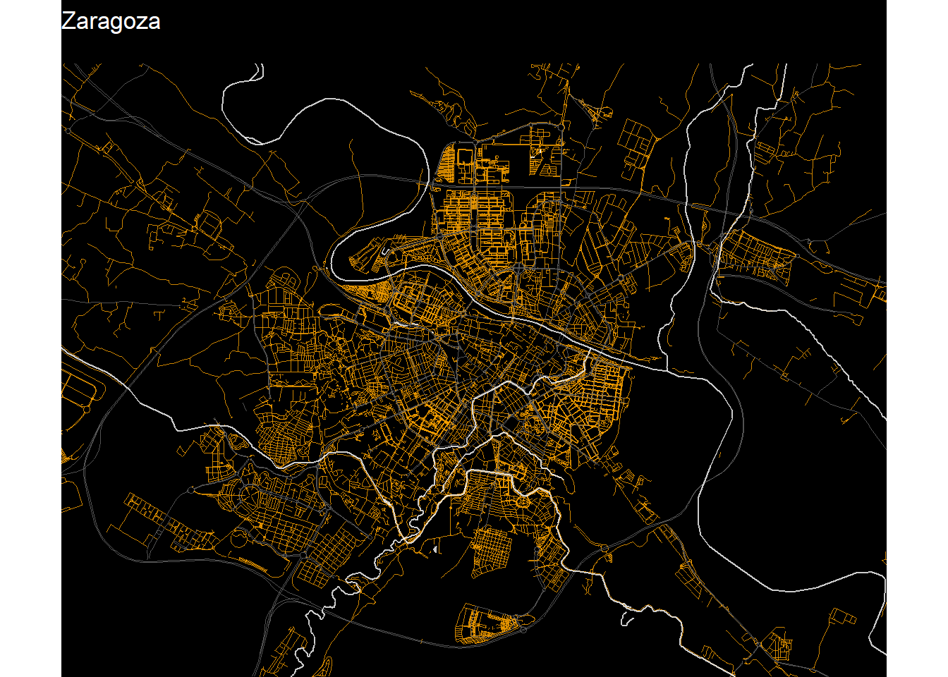

Carriles bici

Zaragoza es una de las ciudades donde el uso de la bicicleta se ha extendido notablemente en los últimos años, tal y como asegura este barómetro de la OCU realizado hace unos años. Tengo curiosidad por comprobar la red de carriles bici existente en la ciudad.

bici <- getbb("Zaragoza Spain")%>%
  opq()%>%
  add_osm_feature(key = "highway", 
                  value = c("cycleway")) %>%
  osmdata_sf()

ggplot() +
 geom_sf(data = calles$osm_lines,
          inherit.aes = FALSE,
          color = "grey30",
          size = .4,
          alpha = .8) +
  geom_sf(data = carreteras$osm_lines,
          inherit.aes = FALSE,
          color = "grey30",
          size = .1,
          alpha = .8) +
  geom_sf(data = bici$osm_lines,
          inherit.aes = FALSE,
          color = "springgreen",
          size = .4,
          alpha = .6) +
  geom_sf(data = rios$osm_lines,
          inherit.aes = FALSE,
          color = "lightblue",
          size = .2,
          alpha = .5) +
  coord_sf(xlim = c(-0.98, -0.8), 
           ylim = c(41.6, 41.7),
           expand = FALSE) +
  theme_void() +
  labs(title = "Zaragoza",
       subtitle = "Carriles bici") +
  theme(plot.background = element_rect(fill = "black"),
        plot.title = element_text(colour = "white"),
        plot.subtitle= element_text(colour = "white"))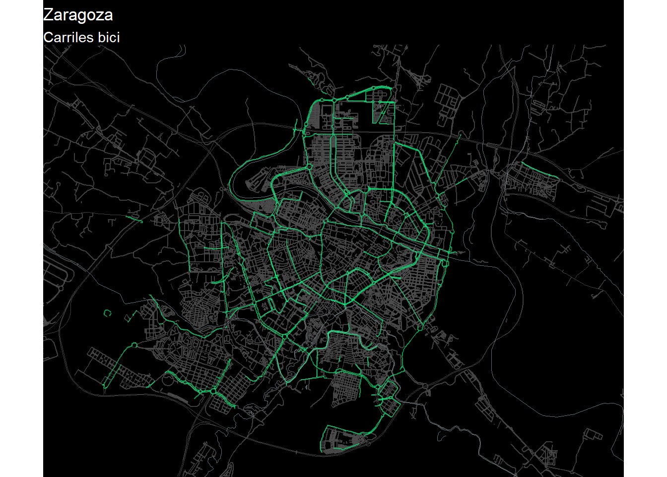

No está mal. Resulta patente que Zaragoza ha apostado por la movilidad sostenible en los últimos años.

Localización de elementos en el mapa

Además de elementos fijos (calles, carriles bici, etc.), OpenStreetMaps nos permite localizar, en un mapa, un gran número de elementos de características diversas. Pongamos por ejemplo que nos interesa identificar y localizar en el mapa de Zaragoza las diferentes sucursales del Banco Santander.

santander <- getbb("Zaragoza Spain")%>%
  opq()%>%
  add_osm_feature("name","Santander")%>%
  add_osm_feature("amenity","bank") %>%
  osmdata_sf()
santander
## Object of class 'osmdata' with:
##                  $bbox : 41.4516625,-1.1737289,41.9314873,-0.6803895
##         $overpass_call : The call submitted to the overpass API
##                  $meta : metadata including timestamp and version numbers
##            $osm_points : 'sf' Simple Features Collection with 0 points
##             $osm_lines : NULL
##          $osm_polygons : 'sf' Simple Features Collection with 0 polygons
##        $osm_multilines : NULL
##     $osm_multipolygons : NULL

ggplot() +
 geom_sf(data = calles$osm_lines,
          inherit.aes = FALSE,
          color = "grey30",
          size = .4,
          alpha = .8) +
  geom_sf(data = carreteras$osm_lines,
          inherit.aes = FALSE,
          color = "grey30",
          size = .1,
          alpha = .8) +
  geom_sf(data = santander$osm_points,
          colour="red",
          fill="red",
          alpha=.6,
          size=2,
          shape=21) +
  geom_sf(data = rios$osm_lines,
          inherit.aes = FALSE,
          color = "lightblue",
          size = .2,
          alpha = .5) +
  coord_sf(xlim = c(-0.98, -0.8), 
           ylim = c(41.6, 41.7),
           expand = FALSE) +
  theme_void() +
  labs(title = "Zaragoza",
       subtitle = "Sucursales del Banco Santander") +
  theme(plot.background = element_rect(fill = "black"),
        plot.title = element_text(colour = "white"),
        plot.subtitle= element_text(colour = "white"))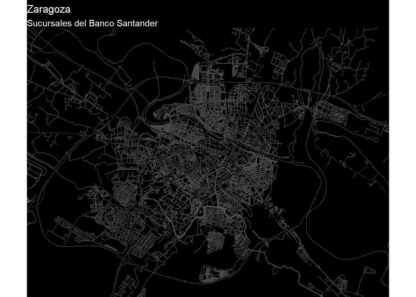

O puede que nos interese identificar en qué lugar se encuentran los distintos estancos en la ciudad:

estancos <- getbb("Zaragoza Spain")%>%
  opq()%>%
  add_osm_feature(key = "shop", 
                  value = "tobacco") %>%
  osmdata_sf()
estancos
## Object of class 'osmdata' with:
##                  $bbox : 41.4516625,-1.1737289,41.9314873,-0.6803895
##         $overpass_call : The call submitted to the overpass API
##                  $meta : metadata including timestamp and version numbers
##            $osm_points : 'sf' Simple Features Collection with 42 points
##             $osm_lines : NULL
##          $osm_polygons : 'sf' Simple Features Collection with 0 polygons
##        $osm_multilines : NULL
##     $osm_multipolygons : NULL

ggplot() +
 geom_sf(data = calles$osm_lines,
          inherit.aes = FALSE,
          color = "grey30",
          size = .4,
          alpha = .8) +
  geom_sf(data = carreteras$osm_lines,
          inherit.aes = FALSE,
          color = "grey30",
          size = .1,
          alpha = .8) +
  geom_sf(data = estancos$osm_points,
          colour="red",
          fill="red",
          alpha=.6,
          size=2,
          shape=21) +
  geom_sf(data = rios$osm_lines,
          inherit.aes = FALSE,
          color = "lightblue",
          size = .2,
          alpha = .5) +
  coord_sf(xlim = c(-0.98, -0.8), 
           ylim = c(41.6, 41.7),
           expand = FALSE) +
  theme_void() +
  labs(title = "Zaragoza",
       subtitle = "Estancos") +
  theme(plot.background = element_rect(fill = "black"),
        plot.title = element_text(colour = "white"),
        plot.subtitle= element_text(colour = "white"))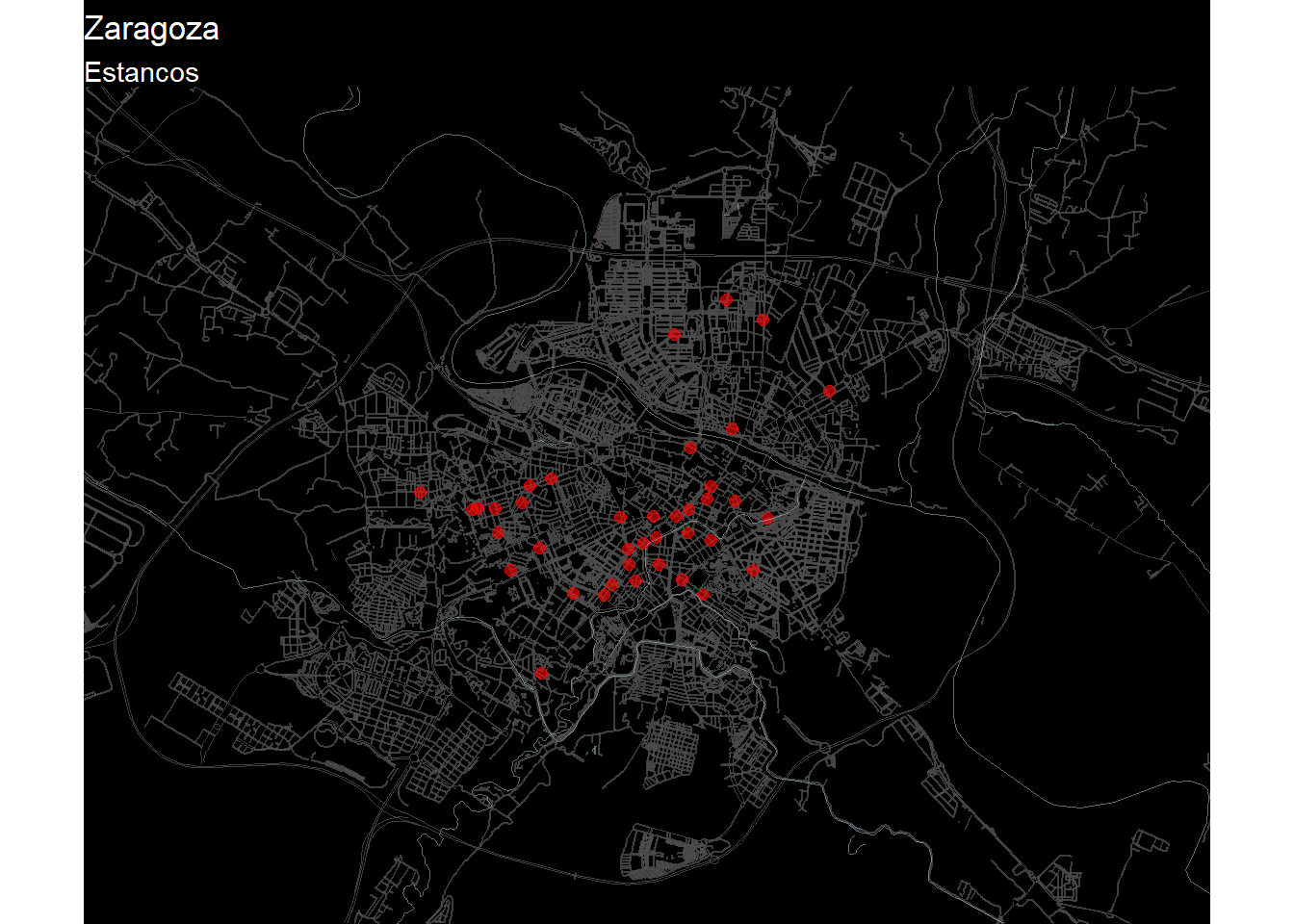

Como no soy usuario habitual de este tipo de establecimientos no sabría decir si la lista de estancos de Zaragoza disponible en OpenStreetMaps se encuentra actualizada o no.

Londres

min <- c(-0.1672, 51.4787)
max <- c(-0.0072, 51.5396)
lnd_df <- as.matrix(data.frame(min, max))
row.names(lnd_df) <- c("x","y")


bike_london_2 <- lnd_df %>%
  opq()%>%
  add_osm_feature(key = "highway", 
                  value = c("cycleway")) %>%
  osmdata_sf()


calles_london_2 <- lnd_df%>%
  opq()%>%
  add_osm_feature(key = "highway", 
                  value = c("residential", "living_street",
                            "unclassified",
                            "service", "footway")) %>%
  osmdata_sf()

ggplot(bike_london_2$osm_lines) +
  geom_sf(colour="orange",
          alpha=.5,
          size=0.5,
          shape=21)+
  geom_sf(data = calles_london_2$osm_lines,
          inherit.aes = F,
          color = "grey40",
          size = .2,
          alpha = .5)+
  theme_void() +
  labs(title = "Londres") +
  theme(plot.background = element_rect(fill = "black"),
        plot.title = element_text(colour = "white", size = 16, hjust = 0.5))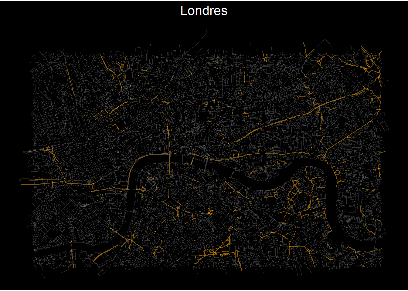

París

min <- c(2.2680, 48.8281)
max <- c(2.4424, 48.8925)
paris_df <- as.matrix(data.frame(min, max))
row.names(paris_df) <- c("x","y")


bike_paris <- paris_df %>%
  opq()%>%
  add_osm_feature(key = "highway", 
                  value = c("cycleway")) %>%
  osmdata_sf()


calles_paris <- paris_df%>%
  opq()%>%
  add_osm_feature(key = "highway", 
                  value = c("residential", "living_street",
                            "unclassified",
                            "service", "footway")) %>%
  osmdata_sf()

ggplot(bike_paris$osm_lines) +
  geom_sf(colour="orange",
          alpha=.5,
          size=0.5,
          shape=21)+
  geom_sf(data = calles_paris$osm_lines,
          inherit.aes = F,
          color = "grey40",
          size = .2,
          alpha = .5)+
  theme_void() +
  labs(title = "Paris") +
  theme(plot.background = element_rect(fill = "black"),
        plot.title = element_text(colour = "white", size = 16, hjust = 0.5))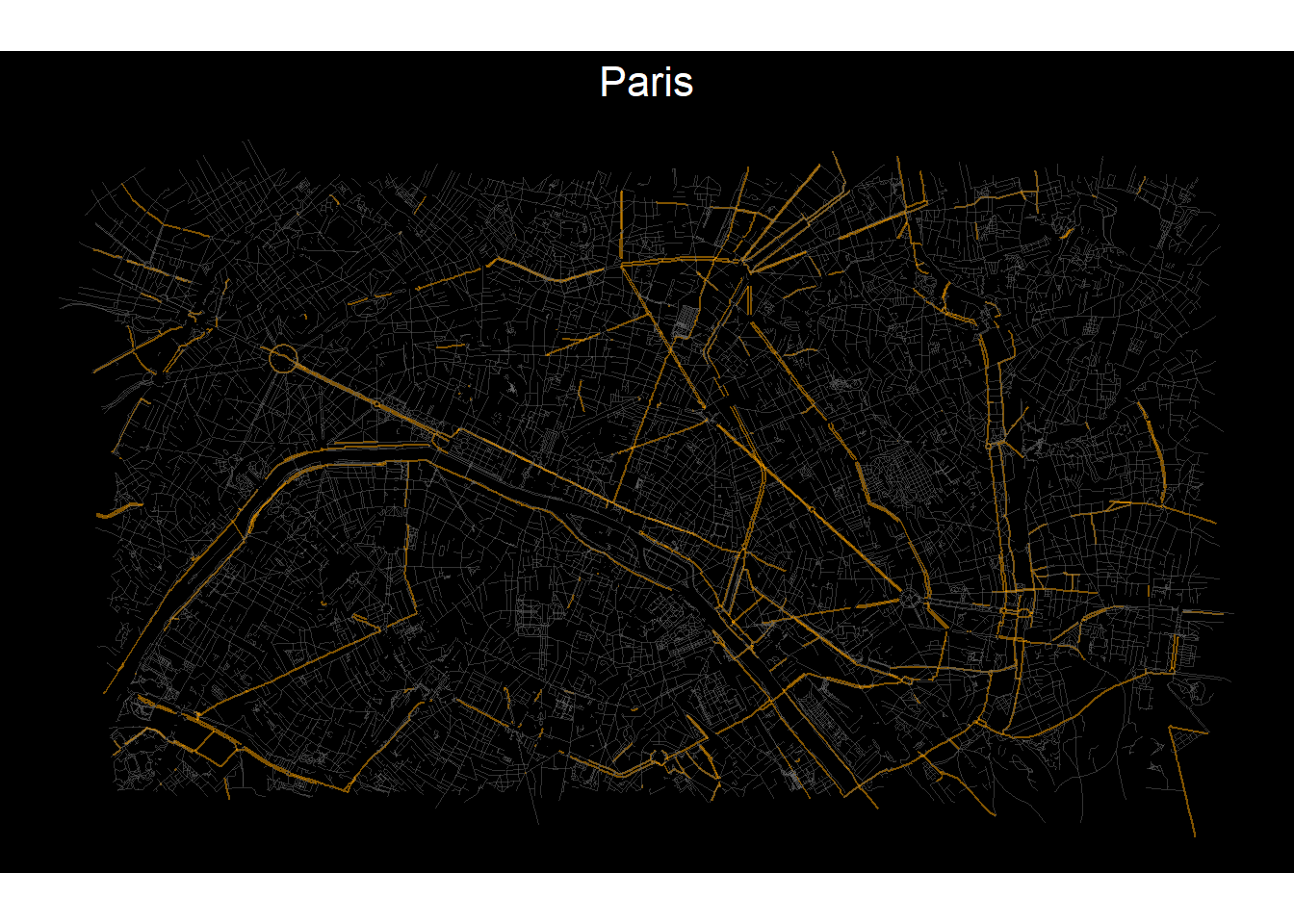

Amsterdam

min <- c(4.8573, 52.3571)
max <- c(4.9445, 52.3870)
amst_df <- as.matrix(data.frame(min, max))
row.names(amst_df) <- c("x","y")


bike_amst <- amst_df %>%
  opq()%>%
  add_osm_feature(key = "highway", 
                  value = c("cycleway")) %>%
  osmdata_sf()


calles_amst <- amst_df%>%
  opq()%>%
  add_osm_feature(key = "highway", 
                  value = c("residential", "living_street",
                            "unclassified",
                            "service", "footway")) %>%
  osmdata_sf()

ggplot(bike_amst$osm_lines) +
  geom_sf(colour="orange",
          alpha=.5,
          size=0.5,
          shape=21)+
  geom_sf(data = calles_amst$osm_lines,
          inherit.aes = F,
          color = "grey40",
          size = .2,
          alpha = .5)+
  theme_void() +
  labs(title = "Amsterdam") +
  theme(plot.background = element_rect(fill = "black"),
        plot.title = element_text(colour = "white", size = 16, hjust = 0.5))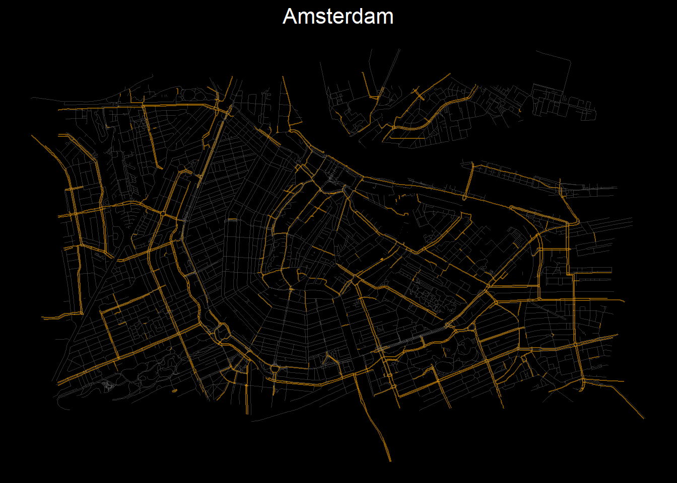

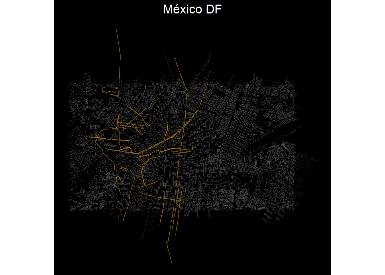
México DF

min <- c(-99.2282, 19.3822)
max <- c(-99.0538, 19.4745)
mex_df <- as.matrix(data.frame(min, max))
row.names(mex_df) <- c("x","y")


bike_mex <- mex_df %>%
  opq()%>%
  add_osm_feature(key = "highway", 
                  value = c("cycleway")) %>%
  osmdata_sf()


calles_mex <- mex_df%>%
  opq()%>%
  add_osm_feature(key = "highway", 
                  value = c("residential", "living_street",
                            "unclassified",
                            "service", "footway")) %>%
  osmdata_sf()

ggplot(bike_mex$osm_lines) +
  geom_sf(colour="orange",
          alpha=.5,
          size=0.5,
          shape=21)+
  geom_sf(data = calles_mex$osm_lines,
          inherit.aes = F,
          color = "grey40",
          size = .2,
          alpha = .5)+
  theme_void() +
  labs(title = "México DF") +
  theme(plot.background = element_rect(fill = "black"),
        plot.title = element_text(colour = "white", size = 16, hjust = 0.5))